Mediation Analysis in R from Scratch (with R code)
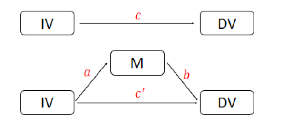
This tutorial shows you how to do mediation analysis in R from scratch. As we know, quantitatively, mediation analysis is about if the product of a*b is statistically significant (see figure below).
If you assume that a*b is normally distributed, you can just directly test the level of significance. If you do not assume normal distribution, you could use quantile or other methods.

Mediation Analysis in R from Scratch
The following is the key, complete R code for the mediation analysis.
library(boot)
set.seed(123)

Mediation_function<-function(data_used,i)
{
# Sample a data
data_temp=data_used[i,]

# a path
result_a<-lm(M~X, data = data_temp)
a<-result_a$coefficients[2]
# b path
result_b<-lm(Y~M+X, data = data_temp)
b<-result_b$coefficients[2]
#calculating the indirect effect
indirect_effect<-a*b
return(indirect_effect)
}

# use boot() to do bootstrapping mediation analysis
boot_mediation <- boot(Mediation_data, Mediation_function, R=5000)

# read data
Mediation_data <-read.csv('https://raw.githubusercontent.com/TidyPython/Mediation_analysis/main/mediation_hypothetical_data.csv')

# show the head of the data
head(Mediation_data)

# print out confidence intervals
boot.ci(boot.out = boot_mediation, type = c("norm", "perc"))
The following is the output. As you can see, it produces the confidence intervals based on normal distribution assumptions and percentile as well. Neither of the confidence intervals includes zero. Thus, we can conclude that the mediation model works. (It should be noted that, the normal distribution assumption is for the 5000 bootstrapping indirect effects.)
BOOTSTRAP CONFIDENCE INTERVAL CALCULATIONS
Based on 5000 bootstrap replicates

CALL :
boot.ci(boot.out = boot_mediation, type = c("norm", "perc"))

Intervals :
Level      Normal             Percentile
95%   ( 0.0377,  0.1570 )   ( 0.0379,  0.1559 )
Calculations and Intervals on Original Scale
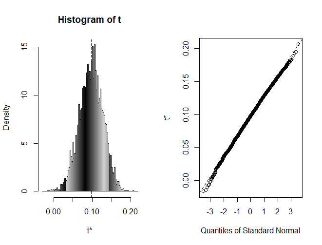
We can also plot the 5000 indirect effects. As we can see, it is pretty normally distributed.
# plot the 5000 indirect effects
plot(boot_mediation)

SE and SD in Bootstrapping Mediation Analysis
Note that, standard error (SE) of a statistic is the standard deviation (SD) of its sampling distribution or an estimate of that standard deviation (based on Wikipedia).
Thus, we can calculate the SE of the indirect effects by calculating the SD of the bootstrapped sample. The following is the R code to show how.
# calculate the standard deviation
sd(boot_mediation$t)
The following is the output:
## [1] 0.03044034
We can double check by printing out the the CI again.
# print out the bootstrapping output again
boot_mediation
The following is the output.
ORDINARY NONPARAMETRIC BOOTSTRAP


Call:
boot(data = Mediation_data, statistic = Mediation_function, R = 5000)


Bootstrap Statistics :
      original       bias    std. error
t1* 0.09748237 0.0001266305  0.03044034
Thus, we can see that SE of the indirect effect is the same as the sd of the bootstrapped sample of indirect effect.
Understand “bias” in the output
The difference between the mean of the bootstrap estimates and the original sample estimate is the bias.
# the mean of 5000 indirect effect
print(mean(boot_mediation$t))
The following is the output:
[1] 0.097609
From the original sample, the following is the output.
#the original sample estimate
print(boot_mediation$t0)
The following is the output:
         X
0.09748237
The difference between these two numbers is the bias.
# the difference = the bias
bias=mean(boot_mediation$t)-boot_mediation$t0
print(bias)
The output:
> print(bias)
           X
0.0001266305
Bias used in Confidence Interval
We can apply this bias in the calculation of CI based on normal distribution assumption.
# calculate the confidence interval from scratch
print(boot_mediation$t0-bias + c(-1, 1) * 1.96 * sd(boot_mediation$t))
The following is the output.
[1] 0.03769268 0.15701880
We can print again the CI from the boot() function.
# print out confidence interval based on normal distribution
boot.ci(boot.out = boot_mediation, type = c("norm"))
The following is the output:
BOOTSTRAP CONFIDENCE INTERVAL CALCULATIONS
Based on 5000 bootstrap replicates

CALL :
boot.ci(boot.out = boot_mediation, type = c("norm"))

Intervals :
Level      Normal
95%   ( 0.0377,  0.1570 )
Calculations and Intervals on Original Scale
We can see that (0.03769268 0.15701880) is the same as ( 0.0377, 0.1570 ), after some rounding up. That means, we need to apply bias when calculate CI based on normal distribution assumption.