Bootstrapping Mediation Analysis in R from Scratch

This tutorial explains how to write code for boostrapping mediation analysis in R from scratch. Mediation analysis is often used in academic research to understand the underlying mechanism. Often, you also need to report a bootstrapping confidence interval for the indirect effect.

Steps of Bootstrapping Mediation Analysis in R

The following shows the steps.

(1) sample a data to estimate path a, and path b, and them time a and b together to get one indirect effect.
(2) Use boot() to repeat 5000 times. Thus, you get 5000 indirect effects.
(3) Use the output from boot() to calculate the confidence intervals.

The following is the flow chart of doing bootstrapping mediation analysis in R from scratch.

R code from Scratch for Bootstrapping Mediation

The following is the complete R code of running bootstrapping mediation analysis in R.

Normal_Mediation<-function(data_used,i)
{
data_temp=data_used[i,]
 # a path 
    result_a_temp<-lm(M~X, data = data_temp)$coefficients
    names(result_a_temp) <- NULL
    a_0_temp<-result_a_temp[1]
    a_1_temp<-result_a_temp[2]
  
 # b path
    result_b_temp<-lm(Y~M+X, data = data_temp)$coefficients
    names(result_b_temp) <- NULL
    b_0_temp<-result_b_temp[1]
    b_1_temp<-result_b_temp[2]
    c_1_apostrophe_temp<-result_b_temp[3]
    
#calculating the indirect effect
    indirect_temp<-a_1_temp*b_1_temp
   return(indirect_temp)
}

#read data from GitHub
Mediation_data <- read.csv('https://raw.githubusercontent.com/TidyPython/Mediation_analysis/main/mediation_hypothetical_data.csv')


set.seed(123)
library(boot)
boot_mediation <- boot(Mediation_data, Normal_Mediation, R=5000)
boot_mediation 

boot.ci(boot.out = boot_mediation, type = c("norm", "basic", "perc", "bca"))

The following is the output. Thus, we can see that the indirect effect is 0.097. The 95% confidence interval based on normal distribution assumption is ( 0.0377, 0.1570 ). The 95% confidence interval using percentile is ( 0.0379, 0.1559 ).

Call:
boot(data = Mediation_data, statistic = Normal_Mediation, R = 5000)


Bootstrap Statistics :
      original       bias    std. error
t1* 0.09748237 0.0001266305  0.03044034
BOOTSTRAP CONFIDENCE INTERVAL CALCULATIONS
Based on 5000 bootstrap replicates

CALL : 
boot.ci(boot.out = boot_mediation, type = c("norm", "basic", 
    "perc", "bca"))

Intervals : 
Level      Normal              Basic         
95%   ( 0.0377,  0.1570 )   ( 0.0391,  0.1571 )  

Level     Percentile            BCa          
95%   ( 0.0379,  0.1559 )   ( 0.0360,  0.1538 )  
Calculations and Intervals on Original Scale

Plot bootstrapping mediation analysis in R

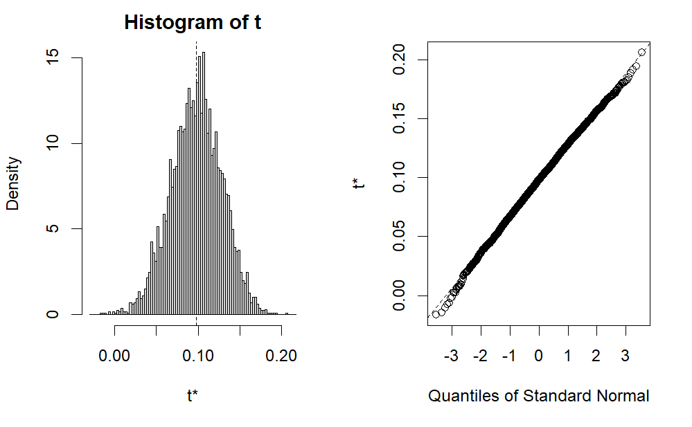
We can also check the distribution of all the indirect effects, which has 5000.

plot(boot_mediation)

The following is the plot of the indirect effect from bootstrapping mediation analysis.

Standard error and standard deviation of bootstrapping

We can also calculate the standard error of the indirect effect. Note that, based on wikipedia, standard error (SE) of a statistic (usually an estimate of a parameter) is the standard deviation of its sampling distribution or an estimate of that standard deviation. Thus, we can just calculate the standard deviation of it.

sd(boot_mediation$t)

The following is the output. It is consistent the output shown above. That is, it is the same as the standard error shown in the “Bootstrap Statistics.”

[1] 0.03044034

Confidence interval functions for bootstrapping from scratch

We can also calcuate the Confidence Interval using our own functions. The following calculates both the normal standard distribution and percentile ones.

 # this is based on normal distribution 
print(boot_mediation$t0 + c(-1, 1) * 1.96 * sd(boot_mediation$t))

 # this is based on percentile 
print(quantile(boot_mediation$t,c(0.025,0.975),type = 6))

The following is the output, which is consitent (but not exactly the same) with the ones shown above.

 # this is based on normal distribution 
[1] 0.03781931 0.15714543

 # this is based on percentile 
     2.5%     97.5% 
0.0378975 0.1558657

Reference

The following UCLA page provides a quick introduction of boot() function.

HOW CAN I GENERATE BOOTSTRAP STATISTICS IN R? | R FAQ

The following is a detailed tutorial about boot() function. It is long but useful.

Understanding Bootstrap Confidence Interval Output from the R boot Package

The following provides a quick introduction of mediation analysis using bootstrapping.

Bootstrapping the Standard Error of the Mediated Effect