Difference between Logit and Probit
This tutorial explains the difference between logit and probit in statistics with formulas and examples.
Formula and Example for Logit
We can start with the following formula.
\[ p(y=1)=\frac{1}{1+e^{-(\beta_0+\beta_1x_1+…+\beta_nx_n)}}=\frac{e^{\beta_0+\beta_1x_1+…+\beta_nx_n}}{1+e^{\beta_0+\beta_1x_1+…+\beta_nx_n}} \]
Thus, \( \beta_0+\beta_1x_1+…+\beta_nx_n \) can be from \( -\infty \) to \(+\infty \), and \( p(y=1) \) will be always within the range of \( (0,1) \).
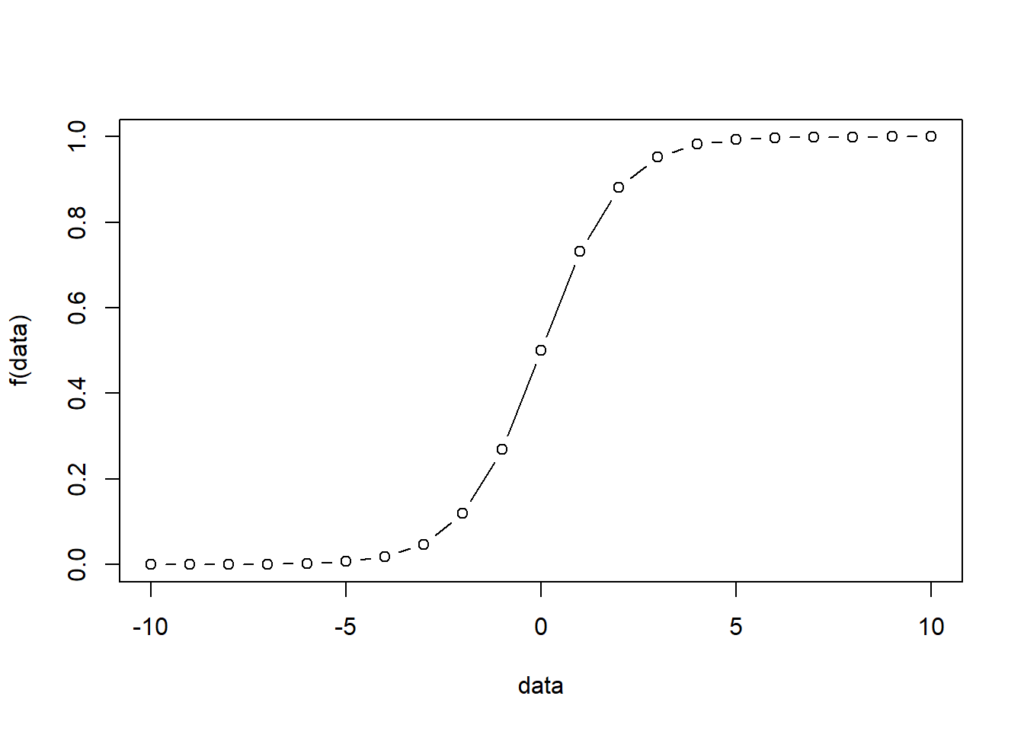
We can use R to illustrate this. The following is the R code and the plot. We can see that the x-axis is from -10 to 10, but the y-axis is in the range of (0,1). Thus, y represents probability.
f<-function(x){exp(x)/(1+exp(x))}
data<-seq(-10,10,1)
plot(data,f(data),type = "b")

We can also rewrite the formula above to another format, namely the log-odds format.
\[ log \frac{p(y=1)}{1-p(y=1)}= \beta_0+\beta_1x_1+…+\beta_nx_n \]
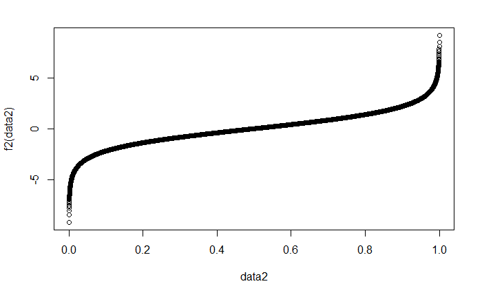
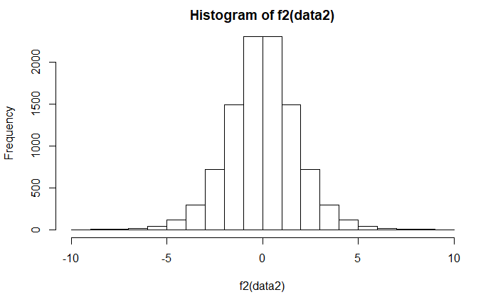
Earlier, we state that \( \beta_0+\beta_1x_1+…+\beta_nx_n \) can be from \( -\infty \) to \(+\infty \). Beyond that, log odds can be in the range of \( -\infty \) to \(+\infty \). Importantly, the distribution of log(odds) can look pretty “normal.”
The following is the R code to illustrate that log(odds) looks pretty normal via a histogram plot.
f2<-function(z){log((z)/(1-z))}
data2<-seq(0,1,0.0001)
plot(data2,f2(data2),type="b")

hist(f2(data2))


After knowing the formula and example of logit, we are going to learn more about probit in the next section. Then, you can understand the connection and difference between these two.
Formula and Example for Probit
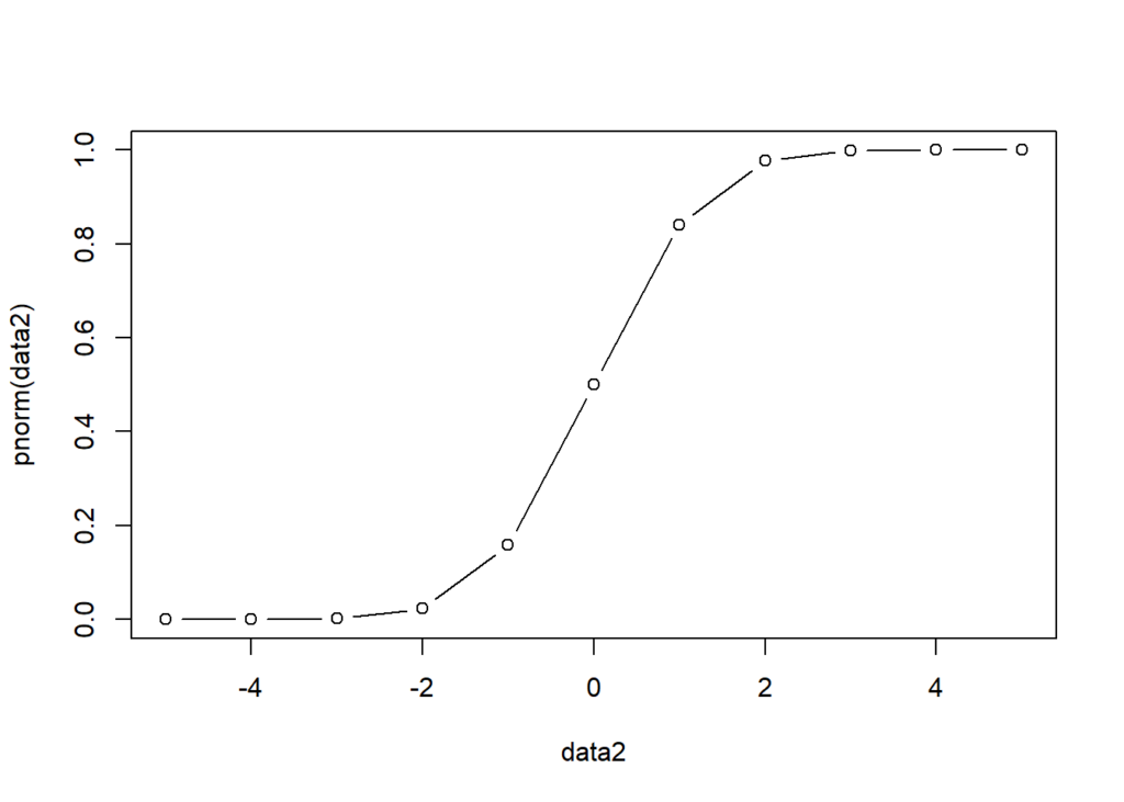
In logit, \( p(y=1)=\frac{1}{1+e^{-(\beta_0+\beta_1x_1+…+\beta_nx_n)}} \) provides the resulting range of (0,1). Another way to provide the same range of (0,1) is through the CDF normal distribution. The following is the CDF standard normal distribution.
\[ CDF=Φ(X)=P(X≤x)={\int_{-\infty }^{x} \frac{1}{\sqrt{2\pi}}}e^{-x^{2}/2}\,dx \]
The following R code is used to illustrate this process.
data2<-seq(-5,5,1)
plot(data2,pnorm(data2),type = "b")

Thus, the CDF of the normal distribution can be used to indicate the probability of \( p(y=1) \).
\[ \Phi(\beta_0+\beta_1x_1+…+\beta_nx_n )= p(y=1) \]
Thus, for instance, \( \beta_0+\beta_1x_1+…+\beta_nx_n \) is -2, we can get that the \( p(y=1)=0.023 \). In contrast, if \( \beta_0+\beta_1x_1+…+\beta_nx_n \) is 3, the \( p(y=1)=0.999 \).
# R code input
pnorm(-2)
pnorm(3)

# R code output
[1] 0.02275013
[1] 0.9986501
Similar to the logit model, we can also write the inverse function of the CDF to get the function that can be from \( -\infty \) to \(+\infty \).
\[ \beta_0+\beta_1x_1+…+\beta_nx_n =\Phi^{-1}(p(y=1)) \]
Conclusion and Further Reading
To conclude, this tutorial provides formulas and examples for logit and probit. Based on these examples, you can see that both logit and probit can be used to analyze binary data. The difference is that logit uses log odds to connect binary DV, whereas probit uses the inverse of CDF.
If you have further questions, please comment down below. If you want to know how to do logistic regression in R, Python, and SPSS, the following are the tutorials. Just note that, logistic regresion typically uses logit, rather than probit.
Discussion