How to Interpret Interaction Effects in Linear Regression (4 Steps)
This tutorial shows how to interpret interaction effects in linear regression models. In summary, there are two perspectives, (a) mean difference perspective and (b) slope difference perspective.
Interpret Interaction Effect in Linear Regression
(a) Mean Difference Perspective:
One way to interpret interaction effects in linear regression is based on mean differences. A significant interaction means that diff13 and diff24 are significantly different.
| IV 2 – Level a | IV 2 – Level b | |
| IV1 – Level a | Cell 1 | Cell 2 |
| IV1 – Level b | Cell 3 | Cell 4 |
| Difference between Levels a and b | diff13=Cell 1-Cell 3 | diff24 = Cell 2-Cell 4 |
(2) Slope Difference Perspective:
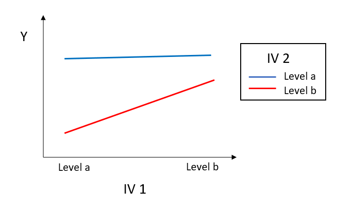
A significant interaction means that the slope of the blue line is significantly different from the slope of the red line.

Steps of Interpretation Interaction Effect in Linear Regression
The following includes steps on how to interpret interaction effects in linear regression models.
Step 1: Prepare for data
Below is the data being used. It has two categorical independent variables (IVs), namely City and Brand. It has one dependent variable, namely sales.
# import the module of pandas
import pandas as pd

# read data from GitHub
df=pd.read_csv("https://raw.githubusercontent.com/TidyPython/interactions/main/city_brand_sales.csv")

# print out the data
print(df)
Output:
     City   Brand  sales
0   City1  brand1     70
1   City1  brand2     10
2   City1  brand1    100
3   City1  brand2      2
4   City1  brand1     30
5   City1  brand2      2
6   City1  brand1     20
7   City1  brand2     10
8   City1  brand1     20
9   City1  brand2     10
10  City2  brand1      9
11  City2  brand2     10
12  City2  brand1      5
13  City2  brand2      4
14  City2  brand1      4
15  City2  brand2      4
16  City2  brand1      5
17  City2  brand2      4
18  City2  brand1     12
19  City2  brand2     11
Step 2: Conduct ANOVA
When the two independent variables are categorical variables, you can use linear regression either or ANOVA as they are the same thing (see my explanation here).
The following uses statsmodels to do linear regression analysis in Python. Since the p-value is 0.023, which is small than 0.05, we can conclude that the interaction is significant.
# import statsmodels
import statsmodels.api as sm
from statsmodels.formula.api import ols

# model statement
model = ols('sales ~ City + Brand + City:Brand', data=df).fit()

# print out the summary
print(model.summary())
Output:
  OLS Regression Results
==============================================================================
Dep. Variable:                  sales   R-squared:                       0.548
Model:                            OLS   Adj. R-squared:                  0.463
Method:                 Least Squares   F-statistic:                     6.462
Date:                Wed, 15 Jun 2022   Prob (F-statistic):            0.00451
Time:                        15:53:16   Log-Likelihood:                -84.089
No. Observations:                  20   AIC:                             176.2
Df Residuals:                      16   BIC:                             180.2
Df Model:                           3
Covariance Type:            nonrobust
=================================================================================================
                                    coef    std err          t      P>|t|      [0.025      0.975]
-------------------------------------------------------------------------------------------------
Intercept                        48.0000      8.104      5.923      0.000      30.820      65.180
City[T.City2]                   -41.0000     11.461     -3.577      0.003     -65.296     -16.704
Brand[T.brand2]                 -41.2000     11.461     -3.595      0.002     -65.496     -16.904
City[T.City2]:Brand[T.brand2]    40.8000     16.208      2.517      0.023       6.441      75.159
==============================================================================
Omnibus:                       13.534   Durbin-Watson:                   1.877
Prob(Omnibus):                  0.001   Jarque-Bera (JB):               14.579
Skew:                           1.193   Prob(JB):                     0.000683
Kurtosis:                       6.436   Cond. No.                         6.85
==============================================================================

Notes:
[1] Standard Errors assume that the covariance matrix of the errors is correctly specified.
Step 3: Mean Difference Perspective
We can calculate the means of 4 cells to understand the meaning of the interaction (see this post regarding how to do so). We can use the following table to better summarize the results.
| Brand 1 | Brand 2 | |
| City 1 | 48.0 | 6.8 |
| City 2 | 7.0 | 6.6 |
| Difference between City 1 and City 2 | 48.0-7.0=41.0 | 6.8-6.6=0.2 |
For Brand 1, the sales difference between City 1 and City 2 is 41.1. For Brand 2, the difference is 0.2. Therefore, a significant interaction means that 0.2 and 41.1 are statistically significant.
Step 4: Slope Difference Perspective
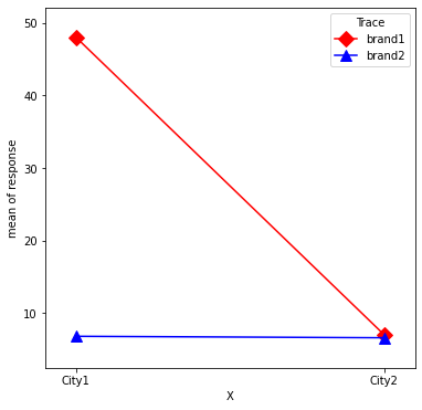
We can also understand interaction from the slope difference perspective. We can plot the interaction below. Regarding how to plot it in Python, please refer to another tutorial.

In particular, the slope for Brand 1 (i.e., the red line) is much steeper than the slope for Brand 2 (i.e., the blue line). Thus, a significant interaction means that these two slopes are significantly different.