How to Use rnorm in R (Examples of Simulate Normal Distribution)
rnorm() in R can be used to simulate a sample of normal distribution data. This tutorial uses 3 examples showing how you can simulate normal distribution sample using rnorm().
In particular, rnorm has the following statement.
rnorm(n, mean=0, sd=1)
- n: The number of observations, namely the sample size
- mean: The mean of the normal distribution sample data. The default value is 0.
- sd: The standard deviation. The default value is 1.
Examples of using rnorm() to simulate normal distribution in R
Example 1:
The following example generates a sample of normal distribution using rnorm. The mean is 5 and sd is 4.
# set seed
set.seed(12)

# create 50 data points, mean = 5, sd=4
X <- rnorm(50, 5, 4)

# print out the data
print(X)

# check mean of the simulated data
print(mean(X))

# check sd of the simulated data
sd(X)

# plot the histogram of the simulated data
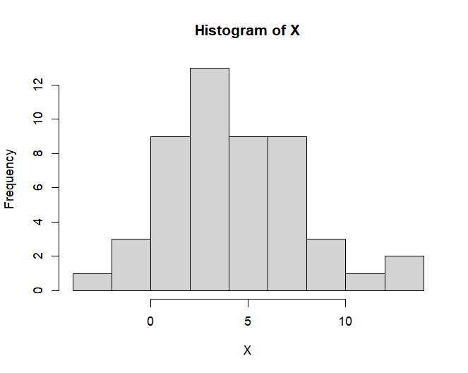
hist(X)
Output:
> # print out the data
> print(X)
 [1] -0.9222704 11.3086779  1.1730221  1.3199790 -2.9905684
 [6]  3.9108158  3.7386052  2.4869791  4.5741445  6.7120592
[11]  1.8891217 -0.1755292  1.8817340  5.0478070  4.3903350
[16]  2.1861430  9.7555166  6.3620491  7.0278727  3.8267794
[21]  5.8945657 13.0288058  9.0479165  3.7901630  0.8990206
[26]  3.9304607  4.2035774  5.5244904  5.5831996  6.4482589
[31]  7.6959247 13.2881431  2.8358854  0.7180314  3.5101731
[36]  3.0594346  6.0991367  3.0819498  8.1924213  0.9821952
[41]  5.4199369  0.3760284  7.3125385 -1.3825026  3.7659854
[46]  6.7978637  1.0917869  5.7599914  7.9258134  3.0296036
>
> # check mean
> print(mean(X))
[1] 4.428281
>
> # check sd
> sd(X)
[1] 3.465599
The mean is 4.42, which is close to 5. The SD is 3.47, which is close to 4. Note that, if you increase the sample size (e.g., 2000), these two values will be closer to the predetermined values.
The following is the histogram plot for the 50 data points in the sample.

Example 2:
You can also use the default values of mean (i.e., 0) and sd (i.e., 1) in rnorm function to simulate a sample of normal distrbution data.
If you use the default mean and sd, you only need to specify the size of the sample, namely the number of data points.
# set seed
set.seed(12)

# create 50 data points, mean = 0, sd=1 (default values)
Y <- rnorm(50)

# print out the data
print(Y)

# check mean of the simulated data
print(mean(X))

# check sd of the simulated data
sd(X)
Output:
> # print out the data
> print(Y)
 [1] -1.48056759  1.57716947 -0.95674448 -0.92000525 -1.99764210
 [6] -0.27229604 -0.31534871 -0.62825524 -0.10646388  0.42801480
[11] -0.77771958 -1.29388230 -0.77956651  0.01195176 -0.15241624
[16] -0.70346425  1.18887916  0.34051227  0.50696817 -0.29330515
[21]  0.22364142  2.00720146  1.01197912 -0.30245925 -1.02524484
[26] -0.26738483 -0.19910566  0.13112260  0.14579990  0.36206472
[31]  0.67398116  2.07203577 -0.54102865 -1.07049216 -0.37245673
[36] -0.48514135  0.27478418 -0.47951256  0.79810533 -1.00445120
[41]  0.10498423 -1.15599289  0.57813463 -1.59562566 -0.30850366
[46]  0.44946592 -0.97705328  0.18999786  0.73145336 -0.49259911
>
> # check mean
> print(mean(Y))
[1] -0.1429296
>
> # check sd
> sd(Y)
[1] 0.8663997
We can see the mean is -0.14, which is close the default value of 0. The SD is 0.87, which is close the default value of 1.
Example 3:
As we can see, Example 2 data is not really close to the true mean (i.e., 0) and SD (i.e., 1). In order to make the simulated data closer to these two true values, we can increase the sample size.
Below, I increased the sample size from 50 to 5000. Since it has so many data points, I am not going to print out the data to save space.
# set seed
set.seed(12)

# create 5000 data points, mean = 0, sd=1 (default values)
Y <- rnorm(5000)

# check mean of the simulated data
print(mean(X))

# check sd of the simulated data
sd(X)
Output:
> set.seed(12)
>
> # create 5000 data points, mean = 0, sd=1 (default values)
> Y <- rnorm(5000)
>
> # check mean
> print(mean(Y))
[1] 0.009787384
>
> # check sd
> sd(Y)
[1] 1.012357
We can see the mean is 0.0098, which is closer the default value of 0. The SD is 1.0124, which is closer the default value of 1. Thus, we can see that increasing sample size does help.