Linear Regression with Categorical Variables in R (4 Steps)
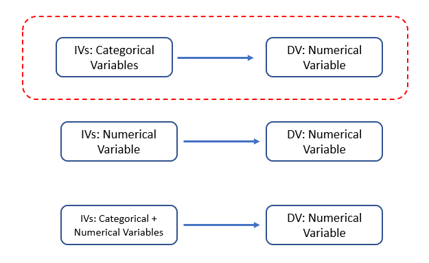
For linear regression models, IVs can be either categorical, numerical, or a combination of them. This tutorial focuses on linear regression with categorical variable as IVs in R.

For instance, the dependent variable Y is sales, whereas the independent variable X is City. City is a categorical variable with two levels, namely City1 and City2.
Sales (Y) = b0 + b1 City (X)
Thus, the linear regression is to estimate the regression coefficents of b0 and b1. The following is the basic syntax of linear regression using lm() in R.
lm(Y~X, data=dataset)
Steps of linear regression with categorical variable
Step 1: Read data into R
We read the data from Github and plan to test the following model. The data shows two categorical variables, City and Brand, and one numerical variable, sales.
df<-read.csv("https://raw.githubusercontent.com/TidyPython/interactions/main/city_brand_sales.csv")

print(df)
Output:
    City  Brand sales
1  City1 brand1    70
2  City1 brand2    10
3  City1 brand1   100
4  City1 brand2     2
5  City1 brand1    30
6  City1 brand2     2
7  City1 brand1    20
8  City1 brand2    10
9  City1 brand1    20
10 City1 brand2    10
11 City2 brand1     9
12 City2 brand2    10
13 City2 brand1     5
14 City2 brand2     4
15 City2 brand1     4
16 City2 brand2     4
17 City2 brand1     5
18 City2 brand2     4
19 City2 brand1    12
20 City2 brand2    11
Step 2: Categorical variable as IV in linear regression model in R
In the following, the categorical variable City is included in the linear regression model as the independent variable (IV), and sales is included as the dependent variable (DV).
The result is saved as estimated_coefficients. We then use the summary() function to print out.
estimated_coefficients <- lm(sales~City, data=df)

summary(estimated_coefficients)
Output:
Call:
lm(formula = sales ~ City, data = df)

Residuals:
   Min     1Q Median     3Q    Max
-25.40  -9.90  -2.80   2.75  72.60

Coefficients:
            Estimate Std. Error t value Pr(>|t|)
(Intercept)   27.400      7.264   3.772   0.0014 **
CityCity2    -20.600     10.273  -2.005   0.0602 .
---
Signif. codes:  0 ‘***’ 0.001 ‘**’ 0.01 ‘*’ 0.05 ‘.’ 0.1 ‘ ’ 1

Residual standard error: 22.97 on 18 degrees of freedom
Multiple R-squared:  0.1826,	Adjusted R-squared:  0.1372
F-statistic: 4.021 on 1 and 18 DF,  p-value: 0.06021
Step 3: Interpretation of linear regression output
We know the estimated b0 and b1 and thus we can insert them into the linear regression model.
Sales = b0 + b1 City = 27.40 – 20.60 City
City uses dummy coding. When City = 0, City represents City1, whereas City =1 represents City2.
- City=0: Sales = 27.40 – 20.60 *0 = 27.40. Thus, sales of City1 is 27.40.
- City=1: Sales = 27.40 – 20.60 *1 = 6.8. Thus, sales of City2 is 6.8.
Step 4: Connection between grouped means and regression coefficents (optional step)
We can also calculate the mean of sales grouped by City. Below is the R code to do so.
# calculate the mean of sales grouped by City
aggregate(df$sales, list(df$City), FUN=mean)
Output:
  Group.1    x
1   City1 27.4
2   City2  6.8
Thus, we can see that intercept b0 is the mean for City1, and coefficient b1 is the mean for City2.