Logistic Regression in R
This tutorial is to show how to do logistic regression in R with examples. The following is the key syntax for logistic regression in R.
glm(Y~ X1 + X2, data = data_frame_name, family = "binomial")
Steps of logistic regression in R
Step 1: Read data and determine model
In this tutorial, we are going to use a dataset posted at UCLA website. It is a hypothetical dataset, and you can download this dataset from their website.
The model we are going to test is as follows.
Log odds of admission (vs. non-admission) = b0+b1 GRE + b2 GPA
Binary_data <- read.csv("https://stats.idre.ucla.edu/stat/data/binary.csv")
head(Binary_data)
Output:
> head(Binary_data)
  admit gre  gpa rank
1     0 380 3.61    3
2     1 660 3.67    3
3     1 800 4.00    1
4     1 640 3.19    4
5     0 520 2.93    4
6     1 760 3.00    2
Step 2: Write out model in R and print out output
The following is the R code to write out model for logistic regression and print out the output.
logit_results <- glm(admit ~ gre + gpa, data = Binary_data, family = "binomial")
summary(logit_results)
Output:
> summary(logit_results)

Call:
glm(formula = admit ~ gre + gpa, family = "binomial", data = Binary_data)

Deviance Residuals:
    Min       1Q   Median       3Q      Max
-1.2730  -0.8988  -0.7206   1.3013   2.0620

Coefficients:
             Estimate Std. Error z value Pr(>|z|)
(Intercept) -4.949378   1.075093  -4.604 4.15e-06 ***
gre          0.002691   0.001057   2.544   0.0109 *
gpa          0.754687   0.319586   2.361   0.0182 *
---
Signif. codes:  0 ‘***’ 0.001 ‘**’ 0.01 ‘*’ 0.05 ‘.’ 0.1 ‘ ’ 1

(Dispersion parameter for binomial family taken to be 1)

    Null deviance: 499.98  on 399  degrees of freedom
Residual deviance: 480.34  on 397  degrees of freedom
AIC: 486.34

Number of Fisher Scoring iterations: 4
Step 3: Write out model and interpret the output of logisitc regression in R
Based on the output in Step 2, we can write out the logistic regression statement as follows.
Log odds of admission (vs. non-admission) = b0+b1 GRE + b2 GPA = -4.949 +0.003 GRE + 0.755 GPA
The interpretations of the logistic regression coefficients are as follows.
- When GRE increases 1 unit, Log odds of admission (vs. non-admission) increases 0.003.
- When GPA increases 1 unit, Log odds of admission (vs. non-admission) increases 0.755.
Step 4 (optional): prediction model for logistic regression in R
We can generate a new set of data to test the result. In particular, we created 10 rows of data with GPA of 4.0 (highest GPA) and 10 rows of data with GPA of 3.39 (mean of GPA)
newdata <- data.frame(gre=rep(seq(from = 220, to = 800, length.out = 10),each=1), gpa = rep(c(max(Binary_data$gpa),mean(Binary_data$gpa)),each=10))

print (newdata)
Output:
> print (newdata)
        gre    gpa
1  220.0000 4.0000
2  284.4444 4.0000
3  348.8889 4.0000
4  413.3333 4.0000
5  477.7778 4.0000
6  542.2222 4.0000
7  606.6667 4.0000
8  671.1111 4.0000
9  735.5556 4.0000
10 800.0000 4.0000
11 220.0000 3.3899
12 284.4444 3.3899
13 348.8889 3.3899
14 413.3333 3.3899
15 477.7778 3.3899
16 542.2222 3.3899
17 606.6667 3.3899
18 671.1111 3.3899
19 735.5556 3.3899
20 800.0000 3.3899
We can also use the estimated model for the new data. Such model will estimate the probability and add them into the data table.
newdata$probability<- predict(logit_results, newdata = newdata, type = "response")
print(newdata)
The following is the updated version of data frame.
> newdata
        gre    gpa probability
1  220.0000 4.0000   0.2077272
2  284.4444 4.0000   0.2377091
3  348.8889 4.0000   0.2705407
4  413.3333 4.0000   0.3060861
5  477.7778 4.0000   0.3440987
6  542.2222 4.0000   0.3842182
7  606.6667 4.0000   0.4259774
8  671.1111 4.0000   0.4688198
9  735.5556 4.0000   0.5121268
10 800.0000 4.0000   0.5552525
11 220.0000 3.3899   0.1419589
12 284.4444 3.3899   0.1644182
13 348.8889 3.3899   0.1896455
14 413.3333 3.3899   0.2177348
15 477.7778 3.3899   0.2487077
16 542.2222 3.3899   0.2824955
17 606.6667 3.3899   0.3189249
18 671.1111 3.3899   0.3577100
19 735.5556 3.3899   0.3984524
20 800.0000 3.3899   0.4406515
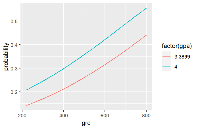
We can further plot it to show the relationship between GRE and probability of getting admitted to graduate schoo. The following is the R code to plot and the actual plot.
library(ggplot2)

ggplot(newdata, aes(x = gre, y = probability))+ geom_line(aes(colour = factor(gpa)))

Appendix: Complete logistic regression in R Code
################################################
# part 1 of logistic regression in R
################################################
# Reading Data
Binary_data <- read.csv("https://stats.idre.ucla.edu/stat/data/binary.csv")
print(Binary_data)


################################################
# part 2 of logistic regression in R
################################################
# logistic model and model summary
logit_results <- glm(admit ~ gre + gpa, data = Binary_data, family = "binomial")
summary(logit_results)


################################################
# part 3 of logistic regression in R
################################################
# oberved data
summary(Binary_data)

# create a new dataframe
newdata <- data.frame(gre=rep(seq(from = 220, to = 800,length.out = 10),each=1),
                      gpa = rep(c(max(Binary_data$gpa),mean(Binary_data$gpa)),each=10))
print (newdata)

# add a new colomn of data
newdata$probability<- predict(logit_results, newdata = newdata, type = "response")
print (newdata)


# plot the data
library(ggplot2)
ggplot(newdata, aes(x = gre, y = probability))+ geom_line(aes(colour = factor(gpa)))