Mediation Analysis for Count Data (with R code)
Warning:
- The correctness and quality of the R code presented in this tutorial are not guaranteed.
- This tutorial is inspired by a paper called “Accommodating binary and count variables in mediation: A case for conditional indirect effects“. However, the author of this tutorial is not one of the authors of that paper.
- The author of this tutorial cannot guarantee that the R code in this tutorial correctly reflects the idea of that paper. Please do read the paper by yourself and make your own judgment.
- Please do NOT cite this tutorial as a reference, if you are writing an academic paper. Further, the author of this tutorial does not provide any consulting service. But, you can leave a comment down below, and I will try my best to help.
Introduction
This tutorial shows how to do mediation analysis for count data in R. Complete R code and examples are provided.
There are two possible ways to consider count data.
(1) You can just assume that the residuals are normally distributed. Then, you can just use the commonly used linear regression model. You can then use Hayes’ PROCESS Macro to do the mediation analysis.
(2) You assume the DV can be fitted into a Poisson distribution, and you can use Poisson regression. In this case, you likely need to write your own program to do the mediation analysis.
Note that, when talking about count data, I mean that DV is count data. The mediator (M) will be still normally distributed, meaning that you can linear regression for a path.
Theoretical Discussion of Mediation for Count Data
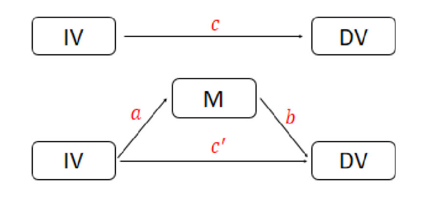
We can estimate \( a \) via a linear regression model since \( M \) is assumed to be normally distributed.
\[ M = a_0 +a_1 IV \]
However, DV is count data and we need to use Poisson regression to estimate \( c \), \( b \), and \( c^{‘} \).
Why do we need to especially consider Poisson regression in mediation analysis? It has something to do with how Poisson constructs its IVs and DV.
\[ DV = exp(b_0+b_1 M + c^{‘} IV)\]
If you calculate the derivative with respect to M, you will get the following.
\[ \frac{\partial DV}{\partial M} = b_1 exp(b_0+b_1 M + c^{‘} IV) \]
Note that, here M is an estimated parameter, given the bootstrapped sample. Thus, we need to calculate based on the following. Thus, it is called conditional indirect effect, since it is based on given \( M \).
\[ \hat{M}= a_0 + a_1 IV \]
Okay, after knowing how to calculate \( \hat{M} \), the problem becomes how to determine \( IV \). This is a bit subjective, as we can either use the mean or +1 /-1 SD of the mean. Thus, you need to predetermine that by yourself and state which one you choose when reporting the mediation result.
The following is the indirect effect.
\[ a_1 * b_1 exp(b_0+b_1 \hat{M} + c^{‘} IV) = a_1 * b_1 exp(b_0+b_1 ( a_0 + a_1 IV )+ c^{‘} IV)\]
Note that, all \( a, b\) are estimated ones, but I do not add \( \hat{} \) on top of them.
Step 1: Mediation Analysis for Count Data
The following is the R code for mediation analysis for count data in R.
library(boot)
set.seed(123)


Mediation_function_poisson<-function(data_used,i,x_predetermined=0)
{
  # Sample a data
  data_temp=data_used[i,]

  # Deciding which X value to use
  if(x_predetermined==0){x_predetermined=mean(data_temp$X)}
  else if (x_predetermined==-1){x_predetermined=mean(data_temp$X)-sd(data_temp$X)}
  else(x_predetermined=mean(data_temp$X)+sd(data_temp$X))

  # a path
  result_a<-lm(M~X, data = data_temp)
  a_0<-result_a$coefficients[1]
  a_1<-result_a$coefficients[2]

    # b path
  result_b<-glm(Y~M+X, data = data_temp, family = quasipoisson)
  b_0<-result_b$coefficients[1]
  b_1<-result_b$coefficients[2]
  c_1_apostrophe<-result_b$coefficients[3]

   #calculating the indirect effect
  M_estimated=a_0+a_1*x_predetermined
  indirect_effect<-a_1*b_1*exp(b_0+b_1*M_estimated+c_1_apostrophe*x_predetermined)
  return(indirect_effect)
}
Step 2: Simulate a dataset with count data for mediation analysis
We can then simulate a dataset to use the function above. The following are the known models. Note that, if you already have the data, you can just read that data into R (thus, you do not need to generate this dataset). You can also just download the dataset I simulated here and skip this step (refer to the code in the appendix of this tutorial to see the download link.).
\[ M= 0.3+0.5 \times X \]
\[ Y = 0.2 + 0.2 \times M+0.08 \times X \]
The following is the R code to simulate the dataset. For more about how to simulate Poisson regression data, you can refer to my other tutorial.
# set the size of the sample
n=500
# set seed
set.seed(123)

# simulate x (normal distribution)
X <- rnorm(n, 5, 4)
# calculate the mean of X
mean_x=mean(X)

# simulate a residual for M
residual_1<-rnorm(n,0,1)
M<-0.3+0.5*X+residual_1

# mu for Poisson regression via a log link
mu_1 <- exp(0.2 + 0.2*M+0.08*X)
# use rpois to generate Y
Y <- rpois(n, lambda=mu_1)

# combine into a dataframe and print out the first 6 rows
data <- data.frame(X=X, M=M, Y=Y)
head(data)
The following are the first 6 rows of the dataset. The full simulated dataset is posted on Github.
> head(data)
          X        M  Y
1  2.758097 1.077156  1
2  4.079290 1.345946  1
3 11.234833 6.944202  8
4  5.282034 3.692078  4
5  5.517151 1.549409  2
6 11.860260 6.134983 17
Step 3: Apply the function in Step 1
In this step, we can apply the function in Step 1.
# use boot() to do bootstrapping mediation analysis
boot_mediation <- boot(data, Mediation_function_poisson, R=1000)
boot_mediation
The following is the output:
> boot_mediation
ORDINARY NONPARAMETRIC BOOTSTRAP

Call:
boot(data = data, statistic = Mediation_function_poisson, R = 1000)

Bootstrap Statistics :
     original       bias    std. error
t1* 0.3352801 0.0009122326  0.03594481
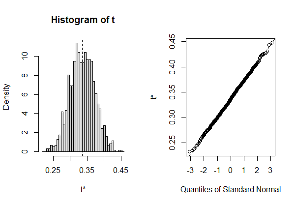
We can also plot the distribution of 1000 indirect. The following is the R code to do so.
# plot the 1000 indirect effects
plot(boot_mediation)
Further, we can print out the confidence intervals for the indirect effect.
# print out confidence intervals
boot.ci(boot.out = boot_mediation, type = c("norm", "perc"))
The following is the output. We can see that the confidence interval based on normal distribution is ( 0.2636, 0.4051 ). For percentile, it is ( 0.2681, 0.4062 ).
> boot.ci(boot.out = boot_mediation, type = c("norm", "perc"))
BOOTSTRAP CONFIDENCE INTERVAL CALCULATIONS
Based on 1000 bootstrap replicates

CALL :
boot.ci(boot.out = boot_mediation, type = c("norm", "perc"))

Intervals :
Level      Normal             Percentile
95%   ( 0.2636,  0.4051 )   ( 0.2681,  0.4062 )
Calculations and Intervals on Original Scale
Step 4: Double check
There are two ways to check if we are on the right track. The first one is that we can check if we can get the exact “original” indirect effect. Note that, “original” is using the whole sample we generated, without any resampling. Thus, we can use the whole sample to test that, and the following is the R code.
# a path
result_a<-lm(M~X, data = data)
a_0<-result_a$coefficients[1]
a_1<-result_a$coefficients[2]
# print out the intercept and regression coefficient
a_0
a_1
The following is the output:
> a_0
(Intercept)
  0.3669984
> a_1
        X
0.4865068
After the a path, we can also calculate the b path as follows.
# b path
result_b<-glm(Y~M+X, data = data, family = poisson(link = log))
b_0<-result_b$coefficients[1]
b_1<-result_b$coefficients[2]
c_1_apostrophe<-result_b$coefficients[3]
# print out the intercept and regression coefficients
b_0
b_1
c_1_apostrophe
The following is the output:
> b_0
(Intercept)
  0.1857203
> b_1
        M
0.2102937
> c_1_apostrophe
         X
0.07752775
Below, we need first calculate the mean of X. Then, we calculate the indirect effect.
#calculating the indirect effect
x_selected=mean(data$X)
# print out the mean of X
x_selected

# calculate the estimated mediator
M_estimated=a_0+a_1*x_selected

# calculate the indirect effect
indirect_effect<-a_1*b_1*exp(b_0+b_1*M_estimated+c_1_apostrophe*x_selected)
indirect_effect
The following is the output. Thus, we can see that we can use the whole sample to calculate the indirect effect and get the exactly same result as from the boot() function output.
> x_selected
[1] 5.138362

> indirect_effect
        X
0.3352801
We can also calculate using the following formula. Note that, I removed some decimals to shorten the formula statement. In order to get the exact 0.3352801, you need to type all the decimals in the output.
\[ a_1 * b_1 exp(b_0+b_1 \hat{M} + c^{‘} IV)= a_1 * b_1 exp(b_0+b_1 ( a_0 + a_1 IV )+ c^{‘} IV) = 0.49 * 0.21 exp(0.19 +0.21* (0.37 +0.49*5.14)+0.0775 *5.14)=0.34\]
We can also calculate the indirect effect based on the theoretical values shown in Step 1. However, since we use randomness in both “residual_1<-rnorm(n,0,1)” and “Y <- rpois(n, lambda=mu_1)“, we are not going to get the exact value.
However, it should be very close. Below, I am going to directly write out the R code calculate statement. Thus, you can copy and paste it into R to check by yourself.
mean_x<-mean(data$X)
theoretical_indirect_effect<-0.5*0.2*exp(0.2+0.2*(0.3+0.5*mean_x)+0.08*mean_x)
theoretical_indirect_effect
The following is the output. We can see that 0.3270377 is pretty close to 0.3352801. That means that our function written above is correct.
> theoretical_indirect_effect
[1] 0.3270377
Further Reading and Discussion
This tutorial is inspired by a paper called “Accommodating binary and count variables in mediation: A case for conditional indirect effects“. You can go to read this article if you want to have a better understanding of mediation analysis for count data. The comment section is open, and if you have any questions, please feel free to comment down below. Your comments will not be shown right away. I will review them as soon as I can and they will appear below if I believe they are not spam and legit questions.
Appendix
The following is the complete R code.
library(boot)
set.seed(123)


Mediation_function_poisson<-function(data_used,i,x_predetermined=0)
{
  # Sample a data
  data_temp=data_used[i,]

  # Deciding which X value to use
  if(x_predetermined==0){x_predetermined=mean(data_temp$X)}
  else if (x_predetermined==-1){x_predetermined=mean(data_temp$X)-sd(data_temp$X)}
  else(x_predetermined=mean(data_temp$X)+sd(data_temp$X))

  # a path
  result_a<-lm(M~X, data = data_temp)
  a_0<-result_a$coefficients[1]
  a_1<-result_a$coefficients[2]

    # b path
  result_b<-glm(Y~M+X, data = data_temp, family = quasipoisson)
  b_0<-result_b$coefficients[1]
  b_1<-result_b$coefficients[2]
  c_1_apostrophe<-result_b$coefficients[3]

   #calculating the indirect effect
  M_estimated=a_0+a_1*x_predetermined
  indirect_effect<-a_1*b_1*exp(b_0+b_1*M_estimated+c_1_apostrophe*x_predetermined)
  return(indirect_effect)
}

# read data from GitHub
data_GitHub <- read.csv(file = 'https://raw.githubusercontent.com/TidyPython/Mediation_analysis/main/data_for_Poission_mediation_analysis.csv')

# use boot() to do bootstrapping mediation analysis
boot_mediation <- boot(data_GitHub, Mediation_function_poisson, R=1000)
boot_mediation

# plot the 1000 indirect effects
plot(boot_mediation)

# print out confidence intervals
boot.ci(boot.out = boot_mediation, type = c("norm", "perc"))
Discussion