Introduction of Normal Distribution Functions in R (Examples)
The tutorial provides examples for each of these 4 normal distribution functions in R. R has 4 normal distribution functions, including rnorm, dnorm, pnorm, and qnorm.
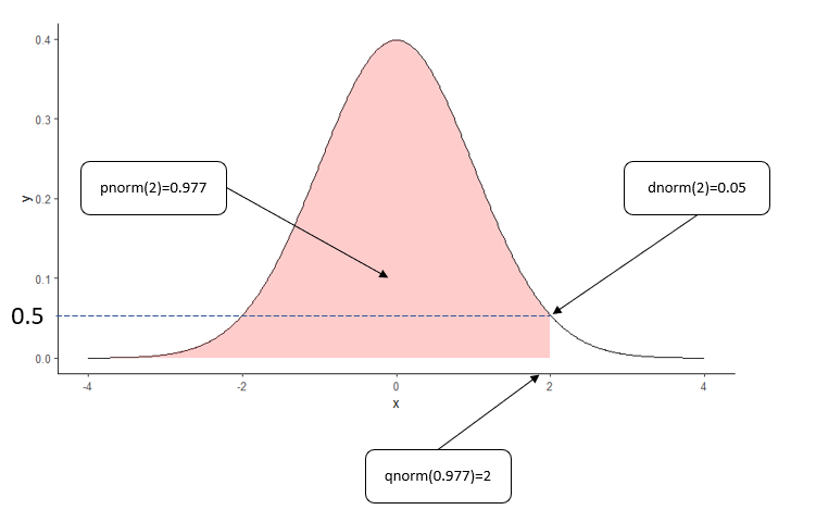
The following table provides a summary for each of these 4 normal distribution functions in R.
| Syntax of R functions | Definitions | Examples |
|---|---|---|
| rnorm(n, mean, sd) | Generate a sample of normal distribution | rnorm(50) returns a sample of 50 data points, with mean = 0 and sd = 1. |
| dnorm(x, mean, sd) | Return the density of probability at point of x | dnorm(2) returns 0.05, which is the density value at point of x=2. |
| pnorm(q, mean, sd) | Return the probabiliy p = CDF value from (-∞, q). | pnorm(2) returns probability p= 0.977. |
| qnorm(p, mean, sd) | Return the quantile value q, based on the probability value of p. | qnorm(0.977) returns the quantile value q= 2. |

Examples of 4 normal distribution functions in R
Example 1: rnorm()
rnorm(50, 2, 4) will generate 50 data points with mean = 2 and sd =4.
The following is the R code of rnorm(50, 2, 4) and its output. It returns a sample of 50 data observations.
> rnorm(50, 2, 4)
 [1] -0.6595560  0.4281984  4.8785564  3.5895556  0.2748618
 [6]  4.8687434  9.5170507  1.5709189  6.8071283  1.4665153
[11]  2.1283960 -3.8310225  1.4255138 -1.6046666  4.3547475
[16] 11.7897579 -1.4176837  8.3676064  5.1467558  0.8026364
[21] 10.6407257  3.0924876  0.5525197  1.4196198  2.7662511
[26]  0.2250933 -2.2283784  9.2073751  4.0276599 -0.6118463
[31]  2.3868138  3.0647955  0.6110670  4.9345245  0.9395610
[36]  2.2158906  4.0917283  4.0740428 -5.4952048 -1.5320750
[41] -0.5265014 -2.3662700  6.3202778 -0.9169152 -2.8141011
[46]  8.1260610  5.7547098 -1.2224999  1.7558709  5.6006177
Example 2: dnorm()
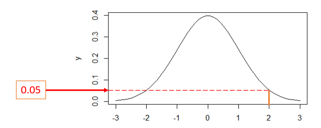
dnorm(2) returns the density of probability at x=2. Note that it is standard normal distribution with mean = 0 and SD = 1.
> dnorm(2)
[1] 0.05399097
We can see that 0.054 is the density of probability at point of 2. Visually, it is the value on Y-axis in the bell shape curve of normal distribution (see the figure below).

Example 3: pnorm()
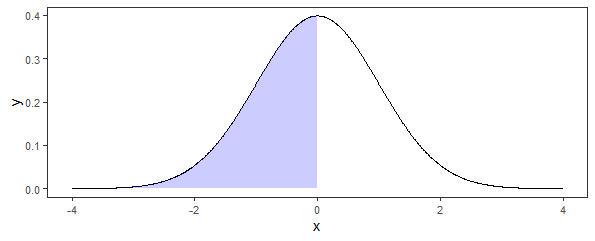
pnorm(0, 0, 1) returns 0.5, which is probability value of the CDF for the range of (-∞, 0) for standard normal distribution (i.e., mean = 0 and sd =1).
> pnorm(0, 0, 1)
[1] 0.5
The following is the plot for pnorm(0, 0, 1). The area of the blue shade is 0.5.

Example 4: qnorm()
qnorm(0.5, 0, 1) returns 0, which is the quantile (i.e., value on the x-axis) for the probability of 0.5. As we can see, qnorm() is just the inverse side of pnorm().
> qnorm(0.5, 0, 1)
[1] 0