Probability Density Functions in R (Examples)
The tutorial shows examples of how you can use built-in Probability Density Functions (PDF) in R, including PDF for normal distribution (dnorm), uniform distribution (dunif), and exponential distribution (dexp).
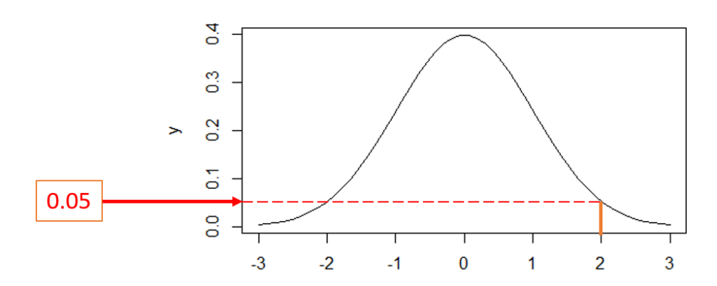
Example 1: PDF for Normal Distribution
Normal distribution PDF dnorm() in R returns the density of probability at 2. Note that it is standard normal distribution with mean = 0 and SD = 1.
> dnorm(2)
[1] 0.05399097
We can see that 0.054 is the density of probability at point of 2. Visually, it is the value on Y-axis in the bell shape curve of normal distribution (see the figure below).
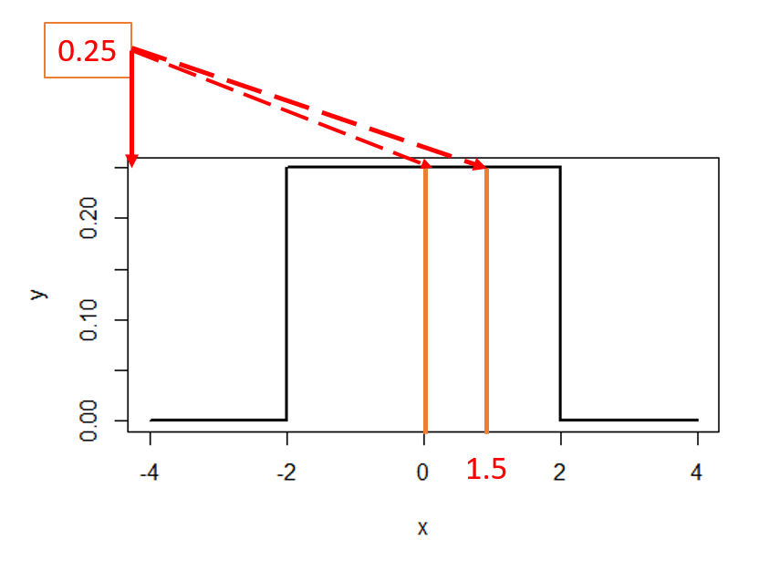
Example 2: PDF for Uniform Distribution
Below, uniform distribution PDF dunif() in R returns the density of probability at x=0 and x=1.5.
> dunif(1.5, min = -2, max = 2)
[1] 0.25
>
> dunif(0, min = -2, max = 2)
[1] 0.25
As we can see above, both of them return 0.25. 0.25 is value on Y-asix corresponding with x=0 and x=1.5. To better understand that, we can plot the PDF function below to see them.
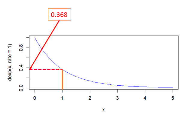
Example 3: PDF for Exponential Distribution
In the following R code, exponential distribution PDF dexp() in R returns the density of probability at x=1.
> dexp(1, rate=1)
[1] 0.3678794
We can see the dexp(1, rate=1) returns 0.368. We can plot it below that 0.368 is the value on Y-asix corresonding with the x=1 for the exponential distribution PDF.