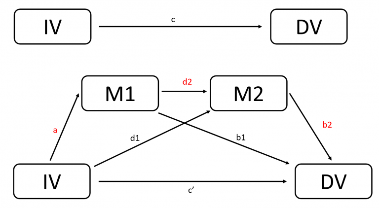
R Code for Serial Mediation
This tutorial shows how you can write R code for serial mediation. Unless you use Hayes’ R code, I am not aware how you can do serial mediation in R. Thus, I am providing this R code here for your convenience.
Note that, the current tutorial is for both mediators and the dependent measure Y are approximately normally distributed. If Y is count data, please refer to my other tutorial.

Step 1 (Optional): Simulate data for serial mediation in R
The following R code simulates a dataset for serial mediation in R. Note that, the data is assumed to follow normal distribution. Further, if you have data already, you can skip this step.
# set sample size
n=1000
# set seed
set.seed(123)

# simulate x (normal distribution), namely IV
X <- rnorm(n, 5, 4)

# simulate residual for M_1
residual_1<-rnorm(n,0,1)
# simulate M_1
M_1<-0.3+0.5*X+residual_1

# simulate residual for M_2
# Note that, residuals for M_1 and M_2 should be different.
# Otherwise, there will be problem of singularities.
residual_2<-rnorm(n,0,1.1)
# simulate M_2
M_2<-0.1+0.7*X+0.5*M_1+residual_2

# simulate residual for Y
residual_3<-rnorm(n,0,1.2)
# simulate Y
Y<-0.5+0.8*X+0.6*M_1+0.9*M_2+residual_3

# combine into a dataframe and print out the first 6 rows
data_normal <- data.frame(X=X, M_1=M_1,M_2=M_2, Y=Y)
head(data_normal)
The following is the output:
> head(data_normal)
          X       M_1       M_2         Y
1  2.758097 0.6832500  1.809529  4.564635
2  4.079290 1.2996900  3.865980  7.629319
3 11.234833 5.8994364 10.318353 20.576248
4  5.282034 2.8088416  6.542995 11.462886
5  5.517151 0.5092327  4.408171 12.304803
6 11.860260 7.2707034 11.360739 24.530397
Step 2: R code for Serial Mediation
The following is the R code for serial mediation, assuming normal distribution.
library(boot)

Serial_Mediation_normal_distribution<-function(data_used,i,x_predetermined=0)
{
  # Sample a data
  data_temp=data_used[i,]

  # Deciding which X value to use
  # Deciding which X value to use
  if(x_predetermined==0){x_predetermined=mean(data_temp$X)}
  else if (x_predetermined==-1){x_predetermined=mean(data_temp$X)-sd(data_temp$X)}
  else(x_predetermined=mean(data_temp$X)+sd(data_temp$X))

  # a path
  result_a<-lm(M_1~X, data = data_temp)
  a_0<-result_a$coefficients[1]
  a_1<-result_a$coefficients[2]

  # d path
  result_d<-lm(M_2~X+M_1, data = data_temp)
  d_0<-result_d$coefficients[1]
  d_1<-result_d$coefficients[2]
  d_2<-result_d$coefficients[3]

  # b path
  result_b<-lm(Y~M_1+M_2+X, data = data_temp)
  b_0<-result_b$coefficients[1]
  b_1<-result_b$coefficients[2]
  b_2<-result_b$coefficients[3]
  c_1_apostrophe<-result_b$coefficients[4]

  #calculating the indirect effect
  indirect_effect<-a_1*d_2*b_2
  return(indirect_effect)
}

# use boot() to do bootstrapping mediation analysis
boot_mediation <- boot(data_normal, Serial_Mediation_normal_distribution, R=1000)
boot_mediation

# print out confidence intervals
boot.ci(boot.out = boot_mediation, type = c("norm", "perc"))
The following is the ouput:
> boot_mediationintervals
ORDINARY NONPARAMETRIC BOOTSTRAP

Call:
boot(data = data_normal, statistic = Serial_Mediation_normal_distribution,
    R = 1000)

Bootstrap Statistics :
     original       bias    std. error
t1* 0.2646659 0.0003075956  0.01911185

> boot.ci(boot.out = boot_mediation, type = c("norm", "perc"))
BOOTSTRAP CONFIDENCE INTERVAL CALCULATIONS
Based on 1000 bootstrap replicates

CALL :
boot.ci(boot.out = boot_mediation, type = c("norm", "perc"))

Intervals :
Level      Normal             Percentile
95%   ( 0.2269,  0.3018 )   ( 0.2276,  0.3061 )
Calculations and Intervals on Original Scale
Step 3 (Optional): Compare with SPSS PROCESS
To verify if our R code is on the right track, I also used SPSS Hayes’ PROCESS Model 6 to check the results. The following is the key output. As we can see, Ind3 is the one that we want to focus, and it is 0.2647, which is the same as 0.2646659 shown in Step 2. Further, we can see the 95% CI is also close.
Indirect effect(s) of X on Y:
          Effect     BootSE   BootLLCI   BootULCI
TOTAL     1.2073      .0315     1.1445     1.2702
Ind1       .2935      .0223      .2502      .3398
Ind2       .6492      .0303      .5878      .7094
Ind3       .2647      .0179      .2301      .3009

Indirect effect key:
Ind1 X           ->    M_1         ->    Y
Ind2 X           ->    M_2         ->    Y
Ind3 X           ->    M_1         ->    M_2         ->    Y
Appendix
Ths is the GitHub link for raw R code for serial mediation analysis, assuming normal distribution. Further, the simulated dataset is also posted on GitHub.