Serial Mediation for Count Data (with R code)
Warning:
- The correctness and quality of the R code presented in this tutorial are not guaranteed.
- This tutorial is inspired by a paper called “Accommodating binary and count variables in mediation: A case for conditional indirect effects“. However, the author of this tutorial is not one of the authors of that paper.
- The author of this tutorial cannot guarantee that the R code in this tutorial correctly reflects the idea of that paper. Please do read the paper by yourself and make your own judgment.
- Please do NOT cite this tutorial as a reference, if you are writing an academic paper. Further, the author of this tutorial does not provide any consulting service. But, you can leave a comment down below, and I will try my best to help.
Introduction
This tutorial shows how to do serial mediation for count data. Complete R code is provided.
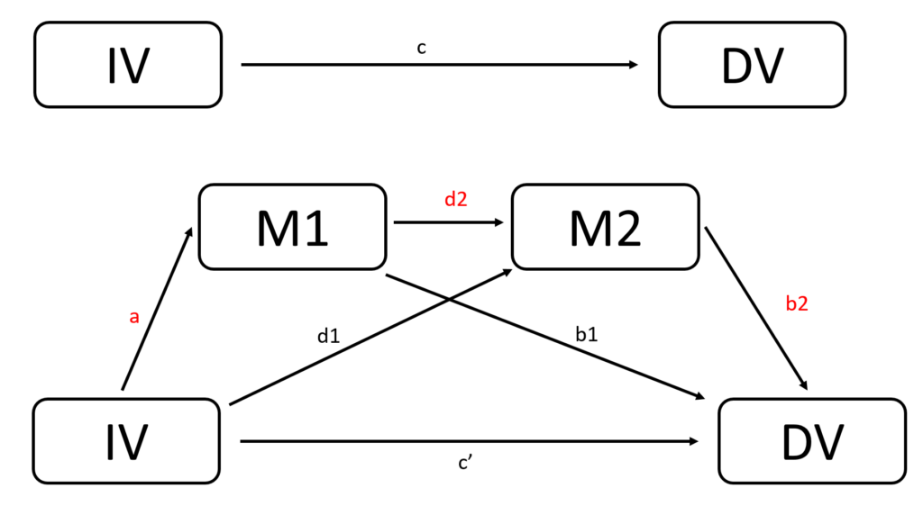
The following are the theoretical models and conceptual framework, assuming IV, M1, M2 are close to normally distributed, and DV is the count data.
\( IV \sim N(4, 5) \)
\( M1 = 0.3+0.5 \times IV \)
\( M2 = 0.1+0.7 \times IV +0.5 \times M1 \)
\( log(E(DV | IV)) = 0.2+0.3 \times M1 +0.3 \times M2 + 0.01 \times IV \)
Step 1 (Optional): Data Simulation
The following is the code to generate the data based on the models stated above. Note that, if you already have data ready, you do not need this simulation step.
# set sample size
n=1000
# set seed
set.seed(123)

# simulate x (normal distribution), namely IV
X <- rnorm(n, 5, 4)

# simulate residual for M_1
residual_1<-rnorm(n,0,1)
# simulate M_1
M_1<-0.3+0.5*X+residual_1

# simulate residual for M_2
# Note that, residuals for M_1 and M_2 should be different.
# Otherwise, there will be problem of singularities.
residual_2<-rnorm(n,0,1.1)
# simulate M_2
M_2<-0.1+0.7*X+0.5*M_1+residual_2

# mu for Poisson regression via a log link
mu_1 <- exp(0.2 + 0.3*M_1+0.3*M_2+0.01*X)
# use rpois to generate Y
Y <- rpois(n, lambda=mu_1)

# combine into a dataframe and print out the first 6 rows
data <- data.frame(X=X, M_1=M_1,M_2=M_2, Y=Y)
Step 2: R code for serial mediation for count data
The following is the R code that can be used to calculate the indirect effect.
library(boot)

Serial_Mediation_poisson<-function(data_used,i,x_predetermined=0)
{
  # Sample a data
  data_temp=data_used[i,]

  # Deciding which X value to use
  if(x_predetermined==0){x_predetermined=mean(data_temp$X)}
  else if (x_predetermined==-1){x_predetermined=mean(data_temp$X)-sd(data_temp$X)}
  else(x_predetermined=mean(data_temp$X)+sd(data_temp$X))

   # a path
  result_a<-lm(M_1~X, data = data_temp)
  a_0<-result_a$coefficients[1]
  a_1<-result_a$coefficients[2]

   # d path
  result_d<-lm(M_2~X+M_1, data = data_temp)
  d_0<-result_d$coefficients[1]
  d_1<-result_d$coefficients[2]
  d_2<-result_d$coefficients[3]

   # b path
  result_b<-glm(Y~M_1+M_2+X, data = data_temp, family = quasipoisson)
  b_0<-result_b$coefficients[1]
  b_1<-result_b$coefficients[2]
  b_2<-result_b$coefficients[3]
  c_1_apostrophe<-result_b$coefficients[4]

   #calculating the indirect effect
  M_1_estimated=a_0+a_1*x_predetermined
  M_2_estimated=d_0+d_1*x_predetermined+d_2*M_1_estimated
  indirect_effect<-a_1*d_2*b_2*exp(b_0+b_1*M_1_estimated+b_2*M_2_estimated+c_1_apostrophe*x_predetermined)
  return(indirect_effect)
}

# use boot() to do bootstrapping mediation analysis
boot_mediation <- boot(data, Serial_Mediation_poisson, R=1000)
boot_mediation

# print out confidence intervals
boot.ci(boot.out = boot_mediation, type = c("norm", "perc"))
The following is the output:
> boot_mediation
ORDINARY NONPARAMETRIC BOOTSTRAP

Call:
boot(data = data, statistic = Serial_Mediation_poisson, R = 1000)

Bootstrap Statistics :
    original      bias
t1*   1.1202 0.006848951
     std. error
t1*   0.1039129

> boot.ci(boot.out = boot_mediation, type = c("norm", "perc"))
BOOTSTRAP CONFIDENCE INTERVAL CALCULATIONS
Based on 1000 bootstrap replicates

CALL :
boot.ci(boot.out = boot_mediation, type = c("norm", "perc"))

Intervals :
Level      Normal             Percentile
95%   ( 0.910,  1.317 )   ( 0.928,  1.341 )
Calculations and Intervals on Original Scale
Step 3 (Optional): Check the model
We can also check the theoretical value of the indirect effect using the following R code. The value is 1.028849. It is not exactly the same as the the value of 1.1202. This is due to three randomness in the data simulation, 2 in the residuals in normal distribution and 1 in the simulation of Poisson data.
x_mean=mean(data$X)
M_1=0.3+0.5*x_mean
M_2=0.1+0.7*x_mean+0.5*M_1
0.5*0.5*0.3*exp(0.2 + 0.3*M_1+0.3*M_2+0.01*x_mean)
Appendix: Raw Code in GitHub
You can click this link for complete raw R code stored in GitHub.