t-distribution Table
Student’s T-Distribution Table
This table shows critical values of the t-distribution for both one-tailed and two-tailed tests.
| df | α = 0.1 | α = 0.05 | α = 0.01 | |||
|---|---|---|---|---|---|---|
| One-Tail | Two-Tail | One-Tail | Two-Tail | One-Tail | Two-Tail | |
| 1 | 3.0777 | 6.3138 | 6.3138 | 12.7062 | 31.8205 | 63.6567 |
| 2 | 1.8856 | 2.9200 | 2.9200 | 4.3027 | 6.9646 | 9.9248 |
| 3 | 1.6377 | 2.3534 | 2.3534 | 3.1824 | 4.5407 | 5.8409 |
| 4 | 1.5332 | 2.1318 | 2.1318 | 2.7764 | 3.7469 | 4.6041 |
| 5 | 1.4759 | 2.0150 | 2.0150 | 2.5706 | 3.3649 | 4.0321 |
| 6 | 1.4398 | 1.9432 | 1.9432 | 2.4469 | 3.1427 | 3.7074 |
| 7 | 1.4149 | 1.8946 | 1.8946 | 2.3646 | 2.9980 | 3.4995 |
| 8 | 1.3968 | 1.8595 | 1.8595 | 2.3060 | 2.8965 | 3.3554 |
| 9 | 1.3830 | 1.8331 | 1.8331 | 2.2622 | 2.8214 | 3.2498 |
| 10 | 1.3722 | 1.8125 | 1.8125 | 2.2281 | 2.7638 | 3.1693 |
| 11 | 1.3634 | 1.7959 | 1.7959 | 2.2010 | 2.7181 | 3.1058 |
| 12 | 1.3562 | 1.7823 | 1.7823 | 2.1788 | 2.6810 | 3.0545 |
| 13 | 1.3502 | 1.7709 | 1.7709 | 2.1604 | 2.6503 | 3.0123 |
| 14 | 1.3450 | 1.7613 | 1.7613 | 2.1448 | 2.6245 | 2.9768 |
| 15 | 1.3406 | 1.7531 | 1.7531 | 2.1314 | 2.6025 | 2.9467 |
| 16 | 1.3368 | 1.7459 | 1.7459 | 2.1199 | 2.5835 | 2.9208 |
| 17 | 1.3334 | 1.7396 | 1.7396 | 2.1098 | 2.5669 | 2.8982 |
| 18 | 1.3304 | 1.7341 | 1.7341 | 2.1009 | 2.5524 | 2.8784 |
| 19 | 1.3277 | 1.7291 | 1.7291 | 2.0930 | 2.5395 | 2.8609 |
| 20 | 1.3253 | 1.7247 | 1.7247 | 2.0860 | 2.5280 | 2.8453 |
| 21 | 1.3232 | 1.7207 | 1.7207 | 2.0796 | 2.5176 | 2.8314 |
| 22 | 1.3212 | 1.7171 | 1.7171 | 2.0739 | 2.5083 | 2.8188 |
| 23 | 1.3195 | 1.7139 | 1.7139 | 2.0687 | 2.4999 | 2.8073 |
| 24 | 1.3178 | 1.7109 | 1.7109 | 2.0639 | 2.4922 | 2.7969 |
| 25 | 1.3163 | 1.7081 | 1.7081 | 2.0595 | 2.4851 | 2.7874 |
| 26 | 1.3150 | 1.7056 | 1.7056 | 2.0555 | 2.4786 | 2.7787 |
| 27 | 1.3137 | 1.7033 | 1.7033 | 2.0518 | 2.4727 | 2.7707 |
| 28 | 1.3125 | 1.7011 | 1.7011 | 2.0484 | 2.4671 | 2.7633 |
| 29 | 1.3114 | 1.6991 | 1.6991 | 2.0452 | 2.4620 | 2.7564 |
| 30 | 1.3104 | 1.6973 | 1.6973 | 2.0423 | 2.4573 | 2.7500 |
| 40 | 1.3031 | 1.6839 | 1.6839 | 2.0211 | 2.4233 | 2.7045 |
| 50 | 1.2987 | 1.6759 | 1.6759 | 2.0086 | 2.4033 | 2.6778 |
| 60 | 1.2958 | 1.6706 | 1.6706 | 2.0003 | 2.3901 | 2.6603 |
| 70 | 1.2938 | 1.6669 | 1.6669 | 1.9944 | 2.3808 | 2.6479 |
| 80 | 1.2922 | 1.6641 | 1.6641 | 1.9901 | 2.3739 | 2.6387 |
| 90 | 1.2910 | 1.6620 | 1.6620 | 1.9867 | 2.3685 | 2.6316 |
| 100 | 1.2901 | 1.6602 | 1.6602 | 1.9840 | 2.3642 | 2.6259 |
| 200 | 1.2858 | 1.6525 | 1.6525 | 1.9719 | 2.3451 | 2.6006 |
| 500 | 1.2832 | 1.6479 | 1.6479 | 1.9647 | 2.3338 | 2.5857 |
| 1000 | 1.2824 | 1.6464 | 1.6464 | 1.9623 | 2.3301 | 2.5808 |
- How to find the critical t-value?
For instance, you know the df=10 (left-most column) and alpha = 0.05 (two-tail), you can then find the critical value of 2.2281.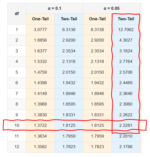
- What does two-tail mean in t-distribution?
Two-tailed means we’re interested in results that could be significantly different in either direction – either unusually high OR unusually low. We split our alpha (significance level) between both tails. You can see the visual example below, where df=10, alpha = 0.05 (two-tail). We can see the critical value of 2.228.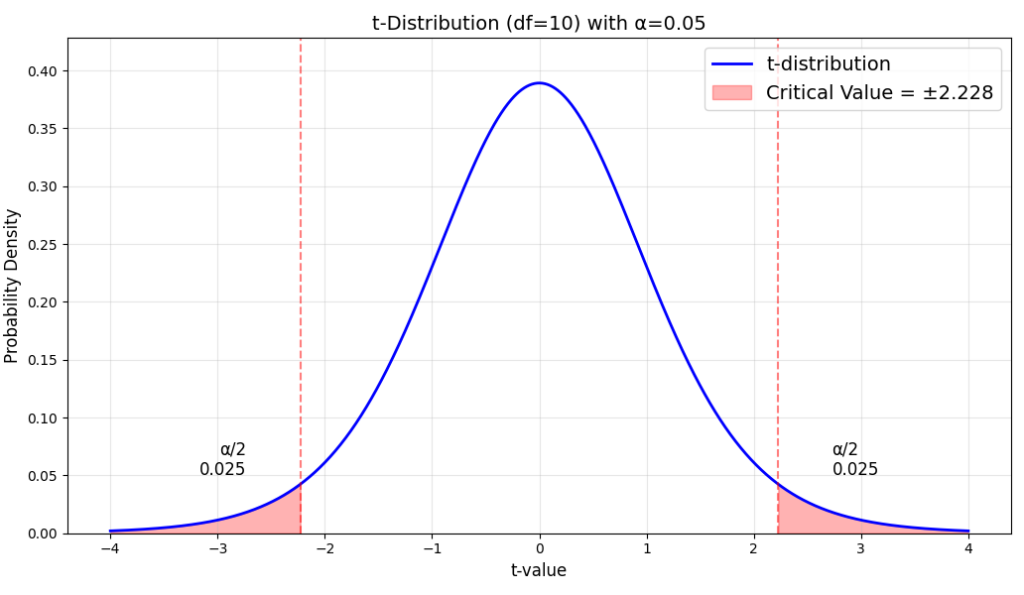
- What does one-tail mean in t-distribution?
In one-tailed tests, we put all of alpha (significance level) in one tail We’re testing if something is either: Significantly GREATER than (right-tailed test) vs. Significantly LESS than (left-tailed test). The following figure is for a right-tailed test. It has df=10, alpha = 0.05 (one-tail), and the critical value of 1.812.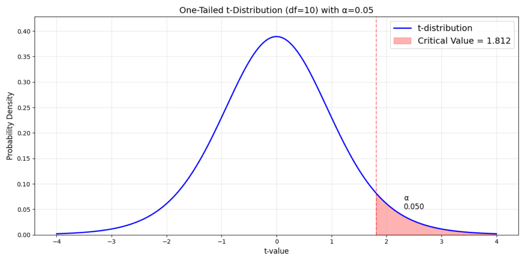
Discussion