Test Normality Assumption for ANOVA in R
This tutorial shows how to test normality assumption for ANOVA in R. I will also highlight mistakes that people tend to make when testing normality.
Math of Normality assumption for ANOVA
Before going to details of how to do that test normality, it is necessary to understand the simple math of testing normality assumption for ANOVA.
Assuming that we have \( k \) groups, and each group has \( n_{i} \) data points. Thus, we can use \( x_{ij} \) to represent data points. Further, we can calculate the mean for each group.
\[ \bar{x_i} =\frac{1}{n_i}\sum_{j=1}^{n_i} x_{ij} \]
Thus, we can calculate the residual, which is each \( x_{ij} \) minus its corresponding group mean \(\bar{x_i} \).
\[ \epsilon_{ij} = x_{ij}-\bar{x_i} \]
Thus, when testing normality assumption, we are testing \( \epsilon_{ij} \), rather than \( x_{ij} \). Sometimes, you will see people make mistakes here.
Step1: Generate the data
We generate a dataset with 3 normal distributions, each with a different mean. In particular, the means are 5, 20, and 30. Each has 30 data points.
# set seed
set.seed(12)
# each group has 30 data points
number_x=30
# combine 3 groups into a dataframe
df <- data.frame(
  Levels=factor(rep(c("X_1", "X_2","X_3"), each=number_x)),
  Measures=round(c(rnorm(number_x, mean=5, sd=2),
                   rnorm(number_x, mean=20, sd=2),
                   rnorm(number_x, mean=30, sd=2))))
# print out first 6 rows of the dataframe
head(df)
The following is the output:
> head(df)
  Levels Measures
1    X_1        2
2    X_1        8
3    X_1        3
4    X_1        3
5    X_1        1
6    X_1        4
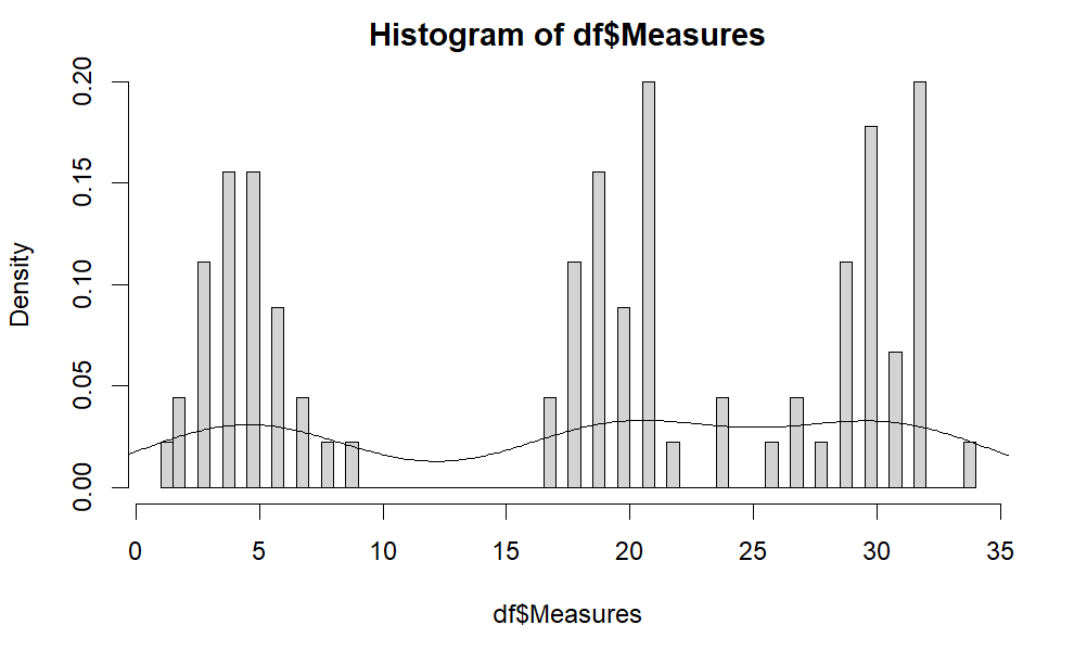
We can also make a histogram to show the overall look of the data. The following are the R code and the histogram. As we can see, there are 3 seperate normal distribution (i.e., 3 bell shapes). Note that, this hisogram is about the distribution of \( x_{ij} \).
hist(df$Measures, freq =FALSE,, breaks = 50)
lines(density(df$Measures))
People sometimes make mistakes to test the normality of \( x_{ij} \). If you do so, you will get the result that \( x_{ij} \) are not normally distributed. In particular, the p-value is 5.956e-07, which is smaller than 0.05. That means \( x_{ij} \) is not normally distributed. Again, this is the wrong way to test normality assumption for ANOVA. Please see Step 2 for the correct way of testing normality assumption for ANOVA.
shapiro.test(df$Measures)

> shapiro.test(df$Measures)
	Shapiro-Wilk normality test

data:  df$Measures
W = 0.88042, p-value = 5.956e-07
Step 2: Use aov() and shapiro.test() to test normality assumption
We can use the combination of aov() and shapiro.test() to test the normality.
model=aov(df$Measures~df$Levels)
res_epsilon=model$residuals
shapiro.test(res_epsilon)
The following is the output. As we can see, the p-value is 0.4124, which is greater than 0.05. Thus, we can conclude that the residuals \( \epsilon_{ij} \) follow normal distribution.
> shapiro.test(res_epsilon)
       Shapiro-Wilk normality test

data:  res_epsilon
W = 0.98538, p-value = 0.4124
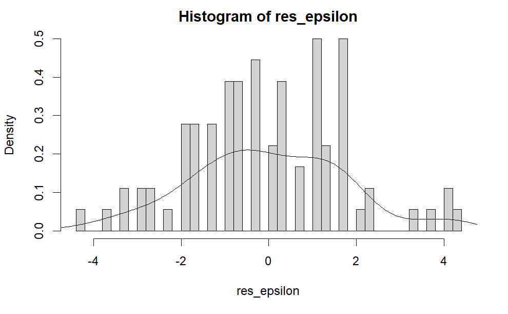
We can also plot the histogram of \( \epsilon_{ij} \) using the following R code.
hist(res_epsilon, freq =FALSE,breaks = 50)
lines(density(res_epsilon))
The following is the output. As we can see, it looks like a single bell shape figure. That is, \( \epsilon_{ij} \) approximately follows a normal distribution. This is different from the histogram of \( x_{ij} \) shown above.