How to Conduct Two-Way ANOVA in R
This tutorial shows how you can do two-way ANOVA in R with examples.
A two-way ANOVA is used to test whether the means from the two or more categorieal variables are significantly different from one another.
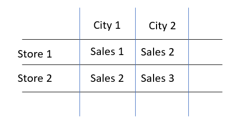
For instance, below, there are two categorical variables, namely city (city 1 and city 2) and store (store 1 and store 2). Suppose that we are interested in comparing whether these 4 sales are significantly different from each other, we can do a two-way ANOVA.

Step 1: Prepare the data for Two-Way ANOVA
The following code generates two categorical variables, x_1 and x_2. Further, it also generates a numerical dependent variable, sales.
x_1 = rep(c('City1','City2'),each=5)
x_2 = rep(c('store1','store2'), 5)
sales=c(10,20,20,50,30,10,5,4,12,4)

df <- data.frame (cities  = x_1,
                  stores = x_2,
                  sales=sales)
Output:
   cities stores sales
1   City1 store1    10
2   City1 store2    20
3   City1 store1    20
4   City1 store2    50
5   City1 store1    30
6   City2 store2    10
7   City2 store1     5
8   City2 store2     4
9   City2 store1    12
10  City2 store2     4
Step 2: Conduct the ANOVA in R
ANOVA function within the package of Companion to Applied Regression (CAR) can be used for the 2-way ANOVA.
The reason of using this one is that we can specify type 2 or type 3 in our analysis (i.e., s type-II or type-III analysis-of-variance tables). In the following, we use type 2.
# Type-II ANOVA in R
car::Anova(lm(sales ~ cities*stores, data = df),type=2)
Output:
Anova Table (Type II tests)

Response: sales
              Sum Sq Df F value  Pr(>F)
cities        984.15  1  8.4537 0.02707 *
stores         93.75  1  0.8053 0.40408
cities:stores 183.75  1  1.5784 0.25569
Residuals     698.50  6
Step 3: Interpret the results of Two-Way ANOVA in R
We need to focus on p-values for the 3 components in the output table.
- p-value for cities: 0.02707 *
- p-value for stores: 0.40408
- p-value for stores for the interaction of cities:stores: 0.25569
First, the p-value for the interaction item of C(cities):C(stores) is 0.256. That means there is no significant interaction effect in the model.
Next, we look at the other two p-values. In particular, the p-value for cities is 0.027, which is smaller than 0.05. Thus, we conclude that city 1 and city 2 differ significantly on sales.
Finally, the p-value for stores is 0.404, which is greater than 0.05, suggesting that store 1 and store 2 do not differ significantly on sales.
Step 4 (Optional): Type 2 vs. Type 3 ANOVA
For the difference between Type 1, Type 2, and Type 3 ANOVA, please refer to my another tutorial on this topic. Let’s see what Type III output looks like.
# Type III ANOVA
car::Anova(lm(sales ~ cities*stores, data = df),type=3)
Output:
Anova Table (Type III tests)

Response: sales
               Sum Sq Df F value  Pr(>F)
(Intercept)   1200.00  1 10.3078 0.01835 *
cities         158.70  1  1.3632 0.28728
stores         270.00  1  2.3193 0.17861
cities:stores  183.75  1  1.5784 0.25569
Residuals      698.50  6
We can see that, cities became insignificant when using Type III ANOVA. In contrast, the interaction item does not change, regardless of using Type II or Type III.
Step 5 (Optional): Remove interaction item
If the intereaction effect is not significant, we actually can remove the interaction item and just include the two factors in the model. (see my discussion here in another tutorial about this. )
Below are the R codes and output doing Type-II ANVOA without the interaction item.
# Type-II ANVOA without the interaction item
car::Anova(lm(sales ~ cities+stores, data = df),type=2)
Output:
Anova Table (Type II tests)

Response: sales
          Sum Sq Df F value  Pr(>F)
cities    984.15  1  7.8085 0.02674 *
stores     93.75  1  0.7438 0.41700
Residuals 882.25  7
Below are the R codes and output doing Type-III ANVOA without the interaction item.
# Type-III ANOVA without the interaction item
car::Anova(lm(sales ~ cities+stores, data = df),type=3)
Output:
Anova Table (Type III tests)

Response: sales
             Sum Sq Df F value   Pr(>F)
(Intercept) 2070.94  1 16.4314 0.004849 **
cities       984.15  1  7.8085 0.026740 *
stores        93.75  1  0.7438 0.417000
Residuals    882.25  7
As we can see above, regardless of using type-II or Type III, the outputs are exactly the same.
This makes sense, since the difference of type-II or Type III is whether to include the interaction item when calculating the main effects. Givent that the model does not include the interaction item, type-II or Type III will be exactly the same.