Z table: Two-tail and One-tail
Two-tail Standard Normal Z-table
Two-tail Standard Normal Z-Table
| |Z| | 0.00 | 0.01 | 0.02 | 0.03 | 0.04 | 0.05 | 0.06 | 0.07 | 0.08 | 0.09 |
|---|---|---|---|---|---|---|---|---|---|---|
| 0.0 | 1.0000 | 0.9920 | 0.9840 | 0.9761 | 0.9681 | 0.9601 | 0.9522 | 0.9442 | 0.9362 | 0.9283 |
| 0.1 | 0.9203 | 0.9124 | 0.9045 | 0.8966 | 0.8887 | 0.8808 | 0.8729 | 0.8650 | 0.8572 | 0.8493 |
| 0.2 | 0.8415 | 0.8337 | 0.8259 | 0.8181 | 0.8103 | 0.8026 | 0.7949 | 0.7872 | 0.7795 | 0.7718 |
| 0.3 | 0.7642 | 0.7566 | 0.7490 | 0.7414 | 0.7339 | 0.7263 | 0.7188 | 0.7114 | 0.7039 | 0.6965 |
| 0.4 | 0.6892 | 0.6818 | 0.6745 | 0.6672 | 0.6599 | 0.6527 | 0.6455 | 0.6384 | 0.6312 | 0.6241 |
| 0.5 | 0.6171 | 0.6101 | 0.6031 | 0.5961 | 0.5892 | 0.5823 | 0.5755 | 0.5687 | 0.5619 | 0.5552 |
| 0.6 | 0.5485 | 0.5419 | 0.5353 | 0.5287 | 0.5222 | 0.5157 | 0.5093 | 0.5029 | 0.4965 | 0.4902 |
| 0.7 | 0.4839 | 0.4777 | 0.4715 | 0.4654 | 0.4593 | 0.4533 | 0.4473 | 0.4413 | 0.4354 | 0.4295 |
| 0.8 | 0.4237 | 0.4179 | 0.4122 | 0.4065 | 0.4009 | 0.3953 | 0.3898 | 0.3843 | 0.3789 | 0.3735 |
| 0.9 | 0.3681 | 0.3628 | 0.3576 | 0.3524 | 0.3472 | 0.3421 | 0.3371 | 0.3320 | 0.3271 | 0.3222 |
| 1.0 | 0.3173 | 0.3125 | 0.3077 | 0.3030 | 0.2983 | 0.2937 | 0.2891 | 0.2846 | 0.2801 | 0.2757 |
| 1.1 | 0.2713 | 0.2670 | 0.2627 | 0.2585 | 0.2543 | 0.2501 | 0.2460 | 0.2420 | 0.2380 | 0.2340 |
| 1.2 | 0.2301 | 0.2263 | 0.2225 | 0.2187 | 0.2150 | 0.2113 | 0.2077 | 0.2041 | 0.2005 | 0.1971 |
| 1.3 | 0.1936 | 0.1902 | 0.1868 | 0.1835 | 0.1802 | 0.1770 | 0.1738 | 0.1707 | 0.1676 | 0.1645 |
| 1.4 | 0.1615 | 0.1585 | 0.1556 | 0.1527 | 0.1499 | 0.1471 | 0.1443 | 0.1416 | 0.1389 | 0.1362 |
| 1.5 | 0.1336 | 0.1310 | 0.1285 | 0.1260 | 0.1236 | 0.1211 | 0.1188 | 0.1164 | 0.1141 | 0.1118 |
| 1.6 | 0.1096 | 0.1074 | 0.1052 | 0.1031 | 0.1010 | 0.0989 | 0.0969 | 0.0949 | 0.0930 | 0.0910 |
| 1.7 | 0.0891 | 0.0873 | 0.0854 | 0.0836 | 0.0819 | 0.0801 | 0.0784 | 0.0767 | 0.0751 | 0.0735 |
| 1.8 | 0.0719 | 0.0703 | 0.0688 | 0.0672 | 0.0658 | 0.0643 | 0.0629 | 0.0615 | 0.0601 | 0.0588 |
| 1.9 | 0.0574 | 0.0561 | 0.0549 | 0.0536 | 0.0524 | 0.0512 | 0.0500 | 0.0488 | 0.0477 | 0.0466 |
| 2.0 | 0.0455 | 0.0444 | 0.0434 | 0.0424 | 0.0414 | 0.0404 | 0.0394 | 0.0385 | 0.0375 | 0.0366 |
| |Z| | 0.00 | 0.01 | 0.02 | 0.03 | 0.04 | 0.05 | 0.06 | 0.07 | 0.08 | 0.09 |
| 2.1 | 0.0357 | 0.0349 | 0.0340 | 0.0332 | 0.0324 | 0.0316 | 0.0308 | 0.0300 | 0.0293 | 0.0285 |
| 2.2 | 0.0278 | 0.0271 | 0.0264 | 0.0257 | 0.0251 | 0.0244 | 0.0238 | 0.0232 | 0.0226 | 0.0220 |
| 2.3 | 0.0214 | 0.0209 | 0.0203 | 0.0198 | 0.0193 | 0.0188 | 0.0183 | 0.0178 | 0.0173 | 0.0168 |
| 2.4 | 0.0164 | 0.0160 | 0.0155 | 0.0151 | 0.0147 | 0.0143 | 0.0139 | 0.0135 | 0.0131 | 0.0128 |
| 2.5 | 0.0124 | 0.0121 | 0.0117 | 0.0114 | 0.0111 | 0.0108 | 0.0105 | 0.0102 | 0.0099 | 0.0096 |
| 2.6 | 0.0093 | 0.0091 | 0.0088 | 0.0085 | 0.0083 | 0.0080 | 0.0078 | 0.0076 | 0.0074 | 0.0071 |
| 2.7 | 0.0069 | 0.0067 | 0.0065 | 0.0063 | 0.0061 | 0.0060 | 0.0058 | 0.0056 | 0.0054 | 0.0053 |
| 2.8 | 0.0051 | 0.0050 | 0.0048 | 0.0047 | 0.0045 | 0.0044 | 0.0042 | 0.0041 | 0.0040 | 0.0039 |
| 2.9 | 0.0037 | 0.0036 | 0.0035 | 0.0034 | 0.0033 | 0.0032 | 0.0031 | 0.0030 | 0.0029 | 0.0028 |
| 3.0 | 0.0027 | 0.0026 | 0.0025 | 0.0024 | 0.0024 | 0.0023 | 0.0022 | 0.0021 | 0.0021 | 0.0020 |
| 3.1 | 0.0019 | 0.0019 | 0.0018 | 0.0017 | 0.0017 | 0.0016 | 0.0016 | 0.0015 | 0.0015 | 0.0014 |
| 3.2 | 0.0014 | 0.0013 | 0.0013 | 0.0012 | 0.0012 | 0.0012 | 0.0011 | 0.0011 | 0.0010 | 0.0010 |
| 3.3 | 0.0010 | 0.0009 | 0.0009 | 0.0009 | 0.0008 | 0.0008 | 0.0008 | 0.0008 | 0.0007 | 0.0007 |
| 3.4 | 0.0007 | 0.0006 | 0.0006 | 0.0006 | 0.0006 | 0.0006 | 0.0005 | 0.0005 | 0.0005 | 0.0005 |
| 3.5 | 0.0005 | 0.0004 | 0.0004 | 0.0004 | 0.0004 | 0.0004 | 0.0004 | 0.0004 | 0.0003 | 0.0003 |
| 3.6 | 0.0003 | 0.0003 | 0.0003 | 0.0003 | 0.0003 | 0.0003 | 0.0003 | 0.0002 | 0.0002 | 0.0002 |
| 3.7 | 0.0002 | 0.0002 | 0.0002 | 0.0002 | 0.0002 | 0.0002 | 0.0002 | 0.0002 | 0.0002 | 0.0002 |
| 3.8 | 0.0001 | 0.0001 | 0.0001 | 0.0001 | 0.0001 | 0.0001 | 0.0001 | 0.0001 | 0.0001 | 0.0001 |
| 3.9 | 0.0001 | 0.0001 | 0.0001 | 0.0001 | 0.0001 | 0.0001 | 0.0001 | 0.0001 | 0.0001 | 0.0001 |
| 4.0 | 0.0001 | 0.0001 | 0.0001 | 0.0001 | 0.0001 | 0.0001 | 0.0000 | 0.0000 | 0.0000 | 0.0000 |
Note: Values represent two-tailed probabilities, P(|Z| ≥ z).
- Hypothesis for Two-tail Z-test
Null Hypothesis: H0 : μ=μ0
Alternate Hypothesis: H1 : μ≠μ0
Decision Criteria: If the absoluate value of z statistic (i.e., |z|) > z critical value then reject the null hypothesis. - Example for Two-tail Z-test
For instance, a manufacturer claims that the average lifetime of a battery is equal to 50 hours and wants to test if that the case. It collects a sample of 40 batteries, finding a sample mean of 48 hours with a standard deviation of 5 hours.
Null Hypothesis: H0 : μ=50
Alternate Hypothesis: H1 : μ≠50
You calculate z value of -2.53 (see below). Based on the table above (|-2.53| = 2.53), we can find that the p-value is 0.0114. Since it is smaller than 0.05, we reject the null hypothesis and conclude that μ≠50.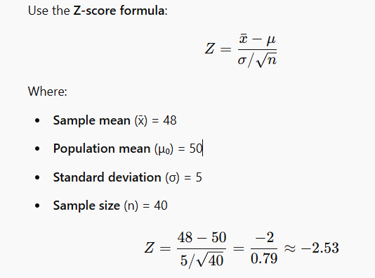
- How can I locate the p-value based on z statistic?
The z-statistic of 2.53 can be broken down into 2.3 + 0.23. Based on that, you can find 0.0114.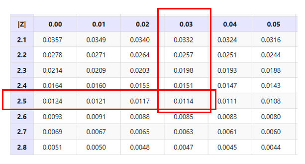
- How can we visually understand the z-statistic and p-value for two-tail z test?
As the name suggests, it has two tails in the bell-shaped curve. The total area of the red regions in both tails is 0.05, with cutoff values of ±1.96. That is, the area of each tail is 0.025. The calculated z-statistic of 2.53 (represented by the green line in the figure below) falls within the rejection region, shaded in red. The rejection region indicates that we need to reject the null hypothesis.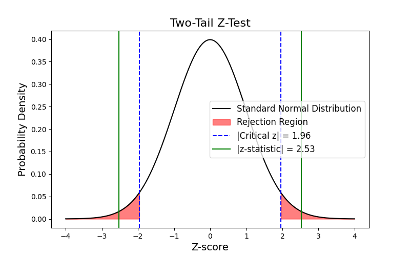
- How do we obtain the value 1.96?
In fact, 1.96 corresponds to a p-value of 0.05. You can locate it in the z-table by adding 1.9 + 0.06. We can also express it as P(|Z| ≥ z) = P(|Z| ≥ 1.96) = 0.05.
One-tail Standard Normal Z-table
One-tail Standard Normal Z-Table
| Left-tail | Right-tail | 0.00 | 0.01 | 0.02 | 0.03 | 0.04 | 0.05 | 0.06 | 0.07 | 0.08 | 0.09 |
|---|---|---|---|---|---|---|---|---|---|---|---|
| -4.0 | 4.0 | 0.0000 | 0.0000 | 0.0000 | 0.0000 | 0.0000 | 0.0000 | 0.0000 | 0.0000 | 0.0000 | 0.0000 |
| -3.9 | 3.9 | 0.0000 | 0.0000 | 0.0000 | 0.0000 | 0.0000 | 0.0000 | 0.0000 | 0.0000 | 0.0000 | 0.0000 |
| -3.8 | 3.8 | 0.0001 | 0.0001 | 0.0001 | 0.0001 | 0.0001 | 0.0001 | 0.0001 | 0.0001 | 0.0001 | 0.0001 |
| -3.7 | 3.7 | 0.0001 | 0.0001 | 0.0001 | 0.0001 | 0.0001 | 0.0001 | 0.0001 | 0.0001 | 0.0001 | 0.0001 |
| -3.6 | 3.6 | 0.0002 | 0.0002 | 0.0001 | 0.0001 | 0.0001 | 0.0001 | 0.0001 | 0.0001 | 0.0001 | 0.0001 |
| -3.5 | 3.5 | 0.0002 | 0.0002 | 0.0002 | 0.0002 | 0.0002 | 0.0002 | 0.0002 | 0.0002 | 0.0002 | 0.0002 |
| -3.4 | 3.4 | 0.0003 | 0.0003 | 0.0003 | 0.0003 | 0.0003 | 0.0003 | 0.0003 | 0.0003 | 0.0003 | 0.0002 |
| -3.3 | 3.3 | 0.0005 | 0.0005 | 0.0005 | 0.0004 | 0.0004 | 0.0004 | 0.0004 | 0.0004 | 0.0004 | 0.0003 |
| -3.2 | 3.2 | 0.0007 | 0.0007 | 0.0006 | 0.0006 | 0.0006 | 0.0006 | 0.0006 | 0.0005 | 0.0005 | 0.0005 |
| -3.1 | 3.1 | 0.0010 | 0.0009 | 0.0009 | 0.0009 | 0.0008 | 0.0008 | 0.0008 | 0.0008 | 0.0007 | 0.0007 |
| -3.0 | 3.0 | 0.0013 | 0.0013 | 0.0013 | 0.0012 | 0.0012 | 0.0011 | 0.0011 | 0.0011 | 0.0010 | 0.0010 |
| -2.9 | 2.9 | 0.0019 | 0.0018 | 0.0018 | 0.0017 | 0.0016 | 0.0016 | 0.0015 | 0.0015 | 0.0014 | 0.0014 |
| -2.8 | 2.8 | 0.0026 | 0.0025 | 0.0024 | 0.0023 | 0.0023 | 0.0022 | 0.0021 | 0.0021 | 0.0020 | 0.0019 |
| -2.7 | 2.7 | 0.0035 | 0.0034 | 0.0033 | 0.0032 | 0.0031 | 0.0030 | 0.0029 | 0.0028 | 0.0027 | 0.0026 |
| -2.6 | 2.6 | 0.0047 | 0.0045 | 0.0044 | 0.0043 | 0.0041 | 0.0040 | 0.0039 | 0.0038 | 0.0037 | 0.0036 |
| -2.5 | 2.5 | 0.0062 | 0.0060 | 0.0059 | 0.0057 | 0.0055 | 0.0054 | 0.0052 | 0.0051 | 0.0049 | 0.0048 |
| -2.4 | 2.4 | 0.0082 | 0.0080 | 0.0078 | 0.0075 | 0.0073 | 0.0071 | 0.0069 | 0.0068 | 0.0066 | 0.0064 |
| -2.3 | 2.3 | 0.0107 | 0.0104 | 0.0102 | 0.0099 | 0.0096 | 0.0094 | 0.0091 | 0.0089 | 0.0087 | 0.0084 |
| -2.2 | 2.2 | 0.0139 | 0.0136 | 0.0132 | 0.0129 | 0.0125 | 0.0122 | 0.0119 | 0.0116 | 0.0113 | 0.0110 |
| -2.1 | 2.1 | 0.0179 | 0.0174 | 0.0170 | 0.0166 | 0.0162 | 0.0158 | 0.0154 | 0.0150 | 0.0146 | 0.0143 |
| -2.0 | 2.0 | 0.0228 | 0.0222 | 0.0217 | 0.0212 | 0.0207 | 0.0202 | 0.0197 | 0.0192 | 0.0188 | 0.0183 |
| Left-tail | Right-tail | 0.00 | 0.01 | 0.02 | 0.03 | 0.04 | 0.05 | 0.06 | 0.07 | 0.08 | 0.09 |
| -1.9 | 1.9 | 0.0287 | 0.0281 | 0.0274 | 0.0268 | 0.0262 | 0.0256 | 0.0250 | 0.0244 | 0.0239 | 0.0233 |
| -1.8 | 1.8 | 0.0359 | 0.0351 | 0.0344 | 0.0336 | 0.0329 | 0.0322 | 0.0314 | 0.0307 | 0.0301 | 0.0294 |
| -1.7 | 1.7 | 0.0446 | 0.0436 | 0.0427 | 0.0418 | 0.0409 | 0.0401 | 0.0392 | 0.0384 | 0.0375 | 0.0367 |
| -1.6 | 1.6 | 0.0548 | 0.0537 | 0.0526 | 0.0516 | 0.0505 | 0.0495 | 0.0485 | 0.0475 | 0.0465 | 0.0455 |
| -1.5 | 1.5 | 0.0668 | 0.0655 | 0.0643 | 0.0630 | 0.0618 | 0.0606 | 0.0594 | 0.0582 | 0.0571 | 0.0559 |
| -1.4 | 1.4 | 0.0808 | 0.0793 | 0.0778 | 0.0764 | 0.0749 | 0.0735 | 0.0721 | 0.0708 | 0.0694 | 0.0681 |
| -1.3 | 1.3 | 0.0968 | 0.0951 | 0.0934 | 0.0918 | 0.0901 | 0.0885 | 0.0869 | 0.0853 | 0.0838 | 0.0823 |
| -1.2 | 1.2 | 0.1151 | 0.1131 | 0.1112 | 0.1093 | 0.1075 | 0.1056 | 0.1038 | 0.1020 | 0.1003 | 0.0985 |
| -1.1 | 1.1 | 0.1357 | 0.1335 | 0.1314 | 0.1292 | 0.1271 | 0.1251 | 0.1230 | 0.1210 | 0.1190 | 0.1170 |
| -1.0 | 1.0 | 0.1587 | 0.1562 | 0.1539 | 0.1515 | 0.1492 | 0.1469 | 0.1446 | 0.1423 | 0.1401 | 0.1379 |
| -0.9 | 0.9 | 0.1841 | 0.1814 | 0.1788 | 0.1762 | 0.1736 | 0.1711 | 0.1685 | 0.1660 | 0.1635 | 0.1611 |
| -0.8 | 0.8 | 0.2119 | 0.2090 | 0.2061 | 0.2033 | 0.2005 | 0.1977 | 0.1949 | 0.1922 | 0.1894 | 0.1867 |
| -0.7 | 0.7 | 0.2420 | 0.2389 | 0.2358 | 0.2327 | 0.2296 | 0.2266 | 0.2236 | 0.2206 | 0.2177 | 0.2148 |
| -0.6 | 0.6 | 0.2743 | 0.2709 | 0.2676 | 0.2643 | 0.2611 | 0.2578 | 0.2546 | 0.2514 | 0.2483 | 0.2451 |
| -0.5 | 0.5 | 0.3085 | 0.3050 | 0.3015 | 0.2981 | 0.2946 | 0.2912 | 0.2877 | 0.2843 | 0.2810 | 0.2776 |
| -0.4 | 0.4 | 0.3446 | 0.3409 | 0.3372 | 0.3336 | 0.3300 | 0.3264 | 0.3228 | 0.3192 | 0.3156 | 0.3121 |
| -0.3 | 0.3 | 0.3821 | 0.3783 | 0.3745 | 0.3707 | 0.3669 | 0.3632 | 0.3594 | 0.3557 | 0.3520 | 0.3483 |
| -0.2 | 0.2 | 0.4207 | 0.4168 | 0.4129 | 0.4090 | 0.4052 | 0.4013 | 0.3974 | 0.3936 | 0.3897 | 0.3859 |
| -0.1 | 0.1 | 0.4602 | 0.4562 | 0.4522 | 0.4483 | 0.4443 | 0.4404 | 0.4364 | 0.4325 | 0.4286 | 0.4247 |
| -0.0 | +0.0 | 0.5000 | 0.4960 | 0.4920 | 0.4880 | 0.4840 | 0.4801 | 0.4761 | 0.4721 | 0.4681 | 0.4641 |
| +0.0 | -0.0 | 0.5000 | 0.5040 | 0.5080 | 0.5120 | 0.5160 | 0.5199 | 0.5239 | 0.5279 | 0.5319 | 0.5359 |
| Left-tail | Right-tail | 0.00 | 0.01 | 0.02 | 0.03 | 0.04 | 0.05 | 0.06 | 0.07 | 0.08 | 0.09 |
| 0.1 | -0.1 | 0.5398 | 0.5438 | 0.5478 | 0.5517 | 0.5557 | 0.5596 | 0.5636 | 0.5675 | 0.5714 | 0.5753 |
| 0.2 | -0.2 | 0.5793 | 0.5832 | 0.5871 | 0.5910 | 0.5948 | 0.5987 | 0.6026 | 0.6064 | 0.6103 | 0.6141 |
| 0.3 | -0.3 | 0.6179 | 0.6217 | 0.6255 | 0.6293 | 0.6331 | 0.6368 | 0.6406 | 0.6443 | 0.6480 | 0.6517 |
| 0.4 | -0.4 | 0.6554 | 0.6591 | 0.6628 | 0.6664 | 0.6700 | 0.6736 | 0.6772 | 0.6808 | 0.6844 | 0.6879 |
| 0.5 | -0.5 | 0.6915 | 0.6950 | 0.6985 | 0.7019 | 0.7054 | 0.7088 | 0.7123 | 0.7157 | 0.7190 | 0.7224 |
| 0.6 | -0.6 | 0.7257 | 0.7291 | 0.7324 | 0.7357 | 0.7389 | 0.7422 | 0.7454 | 0.7486 | 0.7517 | 0.7549 |
| 0.7 | -0.7 | 0.7580 | 0.7611 | 0.7642 | 0.7673 | 0.7704 | 0.7734 | 0.7764 | 0.7794 | 0.7823 | 0.7852 |
| 0.8 | -0.8 | 0.7881 | 0.7910 | 0.7939 | 0.7967 | 0.7995 | 0.8023 | 0.8051 | 0.8078 | 0.8106 | 0.8133 |
| 0.9 | -0.9 | 0.8159 | 0.8186 | 0.8212 | 0.8238 | 0.8264 | 0.8289 | 0.8315 | 0.8340 | 0.8365 | 0.8389 |
| 1.0 | -1.0 | 0.8413 | 0.8438 | 0.8461 | 0.8485 | 0.8508 | 0.8531 | 0.8554 | 0.8577 | 0.8599 | 0.8621 |
| 1.1 | -1.1 | 0.8643 | 0.8665 | 0.8686 | 0.8708 | 0.8729 | 0.8749 | 0.8770 | 0.8790 | 0.8810 | 0.8830 |
| 1.2 | -1.2 | 0.8849 | 0.8869 | 0.8888 | 0.8907 | 0.8925 | 0.8944 | 0.8962 | 0.8980 | 0.8997 | 0.9015 |
| 1.3 | -1.3 | 0.9032 | 0.9049 | 0.9066 | 0.9082 | 0.9099 | 0.9115 | 0.9131 | 0.9147 | 0.9162 | 0.9177 |
| 1.4 | -1.4 | 0.9192 | 0.9207 | 0.9222 | 0.9236 | 0.9251 | 0.9265 | 0.9279 | 0.9292 | 0.9306 | 0.9319 |
| 1.5 | -1.5 | 0.9332 | 0.9345 | 0.9357 | 0.9370 | 0.9382 | 0.9394 | 0.9406 | 0.9418 | 0.9429 | 0.9441 |
| 1.6 | -1.6 | 0.9452 | 0.9463 | 0.9474 | 0.9484 | 0.9495 | 0.9505 | 0.9515 | 0.9525 | 0.9535 | 0.9545 |
| 1.7 | -1.7 | 0.9554 | 0.9564 | 0.9573 | 0.9582 | 0.9591 | 0.9599 | 0.9608 | 0.9616 | 0.9625 | 0.9633 |
| 1.8 | -1.8 | 0.9641 | 0.9649 | 0.9656 | 0.9664 | 0.9671 | 0.9678 | 0.9686 | 0.9693 | 0.9699 | 0.9706 |
| 1.9 | -1.9 | 0.9713 | 0.9719 | 0.9726 | 0.9732 | 0.9738 | 0.9744 | 0.9750 | 0.9756 | 0.9761 | 0.9767 |
| 2.0 | -2.0 | 0.9772 | 0.9778 | 0.9783 | 0.9788 | 0.9793 | 0.9798 | 0.9803 | 0.9808 | 0.9812 | 0.9817 |
| 2.1 | -2.1 | 0.9821 | 0.9826 | 0.9830 | 0.9834 | 0.9838 | 0.9842 | 0.9846 | 0.9850 | 0.9854 | 0.9857 |
| Left-tail | Right-tail | 0.00 | 0.01 | 0.02 | 0.03 | 0.04 | 0.05 | 0.06 | 0.07 | 0.08 | 0.09 |
| 2.2 | -2.2 | 0.9861 | 0.9864 | 0.9868 | 0.9871 | 0.9875 | 0.9878 | 0.9881 | 0.9884 | 0.9887 | 0.9890 |
| 2.3 | -2.3 | 0.9893 | 0.9896 | 0.9898 | 0.9901 | 0.9904 | 0.9906 | 0.9909 | 0.9911 | 0.9913 | 0.9916 |
| 2.4 | -2.4 | 0.9918 | 0.9920 | 0.9922 | 0.9925 | 0.9927 | 0.9929 | 0.9931 | 0.9932 | 0.9934 | 0.9936 |
| 2.5 | -2.5 | 0.9938 | 0.9940 | 0.9941 | 0.9943 | 0.9945 | 0.9946 | 0.9948 | 0.9949 | 0.9951 | 0.9952 |
| 2.6 | -2.6 | 0.9953 | 0.9955 | 0.9956 | 0.9957 | 0.9959 | 0.9960 | 0.9961 | 0.9962 | 0.9963 | 0.9964 |
| 2.7 | -2.7 | 0.9965 | 0.9966 | 0.9967 | 0.9968 | 0.9969 | 0.9970 | 0.9971 | 0.9972 | 0.9973 | 0.9974 |
| 2.8 | -2.8 | 0.9974 | 0.9975 | 0.9976 | 0.9977 | 0.9977 | 0.9978 | 0.9979 | 0.9979 | 0.9980 | 0.9981 |
| 2.9 | -2.9 | 0.9981 | 0.9982 | 0.9982 | 0.9983 | 0.9984 | 0.9984 | 0.9985 | 0.9985 | 0.9986 | 0.9986 |
| 3.0 | -3.0 | 0.9987 | 0.9987 | 0.9987 | 0.9988 | 0.9988 | 0.9989 | 0.9989 | 0.9989 | 0.9990 | 0.9990 |
| 3.1 | -3.1 | 0.9990 | 0.9991 | 0.9991 | 0.9991 | 0.9992 | 0.9992 | 0.9992 | 0.9992 | 0.9993 | 0.9993 |
| 3.2 | -3.2 | 0.9993 | 0.9993 | 0.9994 | 0.9994 | 0.9994 | 0.9994 | 0.9994 | 0.9995 | 0.9995 | 0.9995 |
| 3.3 | -3.3 | 0.9995 | 0.9995 | 0.9995 | 0.9996 | 0.9996 | 0.9996 | 0.9996 | 0.9996 | 0.9996 | 0.9997 |
| 3.4 | -3.4 | 0.9997 | 0.9997 | 0.9997 | 0.9997 | 0.9997 | 0.9997 | 0.9997 | 0.9997 | 0.9997 | 0.9998 |
| 3.5 | -3.5 | 0.9998 | 0.9998 | 0.9998 | 0.9998 | 0.9998 | 0.9998 | 0.9998 | 0.9998 | 0.9998 | 0.9998 |
| 3.6 | -3.6 | 0.9998 | 0.9998 | 0.9999 | 0.9999 | 0.9999 | 0.9999 | 0.9999 | 0.9999 | 0.9999 | 0.9999 |
| 3.7 | -3.7 | 0.9999 | 0.9999 | 0.9999 | 0.9999 | 0.9999 | 0.9999 | 0.9999 | 0.9999 | 0.9999 | 0.9999 |
| 3.8 | -3.8 | 0.9999 | 0.9999 | 0.9999 | 0.9999 | 0.9999 | 0.9999 | 0.9999 | 0.9999 | 0.9999 | 0.9999 |
| 3.9 | -3.9 | 1.0000 | 1.0000 | 1.0000 | 1.0000 | 1.0000 | 1.0000 | 1.0000 | 1.0000 | 1.0000 | 1.0000 |
| 4.0 | -4.0 | 1.0000 | 1.0000 | 1.0000 | 1.0000 | 1.0000 | 1.0000 | 1.0000 | 1.0000 | 1.0000 | 1.0000 |
Note:
- For left-tail tests, the table provides
P(Z ≤ z). - For right-tail tests, the table provides
P(Z ≥ z). - At
z = 0, both negative and positive increments are listed in separate rows. - Z values of the second decimal are repeated in the table several times with purple background color.
One-tail z-test (left-tail)
- Hypothesis for left-tail Z-test
Null Hypothesis: H0 : μ=μ0
Alternate Hypothesis: H1 : μ<μ0
Decision Criteria: If the z statistic < z critical value then reject the null hypothesis. - Example for left-tail Z-test
For instance, a manufacturer claims that the average lifetime of a battery is equal to 50 hours. A researcher believes it’s actually less than 50 hours.
Null Hypothesis: H0 : μ=50
Alternate Hypothesis: H1 : μ < 50
The researcher collects a sample of 40 batteries, finding a sample mean of 48 hours with a standard deviation of 5 hours. The researcher calculates z value of -2.53 (same formula as the two-tail z test), and based on the table above we can find the p-value of 0.0057. Since it is smaller than 0.05, we reject the null hypothesis and conclude that μ < 50. - How can we visually understand the z-statistic and p-value for left-tail z test?
The formula for calculating the p-value for a left-tail z-test is P(Z < z). This means the region starts from negative infinity to a cutoff point of -1.64. Any z-statistic that falls within this red-shaded area indicates that we need to reject the null hypothesis. Since the z-statistic is -2.53 (represented by the green line), we reject the null hypothesis and conclude that μ < 50.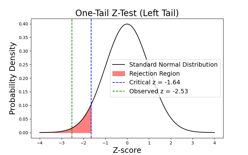
- How do we get the value -1.64, and what does it mean?
The value -1.64 corresponds to P(Z < -1.64) = 0.05, meaning that 5% of the distribution lies to the left of -1.64.
To find -1.64 in the z-table: Locate -1.6 in the leftmost column. Find 0.04 in the top row. The intersection of these values gives 0.0505, which is very close to 0.05. Since the z-table does not list every possible decimal, -1.64 is an approximation commonly used for a one-tailed test at α = 0.05.
One-tail z-test (right-tail)
- Hypothesis for right-tail Z-test
Null Hypothesis: H0 : μ=μ0
Alternate Hypothesis: H1 : μ>μ0
Decision Criteria: If the z statistic > z critical value then reject the null hypothesis. - Example for right-tail Z-test
For instance, a manufacturer claims that the average lifetime of a battery is equal to 50 hours. A researcher believes it’s actually greater than 50 hours.
Null Hypothesis: H0 : μ=50
Alternate Hypothesis: H1 : μ > 50
The researcher collects a sample of 40 batteries, finding a sample mean of 48 hours with a standard deviation of 5 hours. The researcher calculates z value of -2.53 (same formula as before), and based on the table above we can find the p-value of 0.9943. Since it is smaller than 0.05, we fail to reject the null hypothesis. - How can we visually understand the z-statistic and p-value for right-tail z test?
The formula for calculating the p-value for a right-tail z-test is P(Z > z). This means the region starts from positive infinity to a cutoff point of 1.64. Any z-statistic that falls within this red-shaded area indicates that we need to reject the null hypothesis. Since the z-statistic is -2.53 (represented by the green line), we fail to reject the null hypothesis.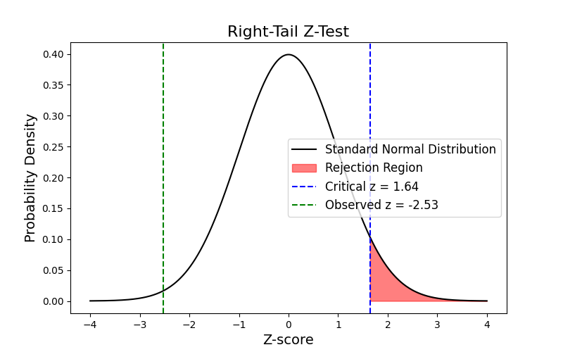
- How do we get the value 1.64 in a right-tailed z-test, and what does it mean?
The value 1.64 corresponds to P(Z > 1.64) = 0.05, meaning that 5% of the distribution lies to the right of 1.64.
To find 1.64 in the z-table. Locate 1.6 in the second leftmost column. Find 0.04 in the top row. The intersection gives 0.0505, which is the same value (and same spot) as in the left-tail z-test.
Note that the one-tailed z-table shown on this page differs from most other sources because it provides both right-tail and left-tail values. Therefore, you do not need to recalculate the right-tail z-score based on a left-tail z-table.
Note that, most online z-tables typically present only left-tail values. For instance, you can click to check this z-table posted on University of Florida website. This table is only provides left-tail z-test scores. In contrast, this page provides z-table for both left-tail and right-tail.
Discussion