Calculate Sample Size for Chi-square Test
This tutorial shows how you can calcuate sample size for one variable chi-square test here.
The example in this tutorial is that a marketing agency tests two versions of packaging (A version vs. B Version). The null hypothesis is that there is no difference between these two versions, and the alternative hypothesis is that there is a difference.
Method 1: R
We can ues R function to do the sample size calculation. The following is the syntax
pwr.chisq.test(w=, N=, df=, sig.level= , power=)
Where,
- W = Effect size
- N = Sample Size (if skipped, it will return the needed sample size.)
- df = degree of freedom
- sig.level=typically 0.05
- power = power to detect the effect
Since we only have two levels (A version vs. B version), the degree of freedom = 1 (2-1=1). We assume that we know the effect size is 0.3. Finally, we set the power to be 0.8.
From the output, we need to have a sample size of 88 (87.21) to have a power of 0.8 to detect the effect, if there is really an effect.
library("pwr")
pwr.chisq.test(w=0.3, df=1, sig.level=0.05,power = 0.8)
> pwr.chisq.test(w=0.3, df=1, sig.level=0.05,power = 0.8)
Chi squared power calculation
w = 0.3
N = 87.20954
df = 1
sig.level = 0.05
power = 0.8
NOTE: N is the number of observations
Method 2: G*Power
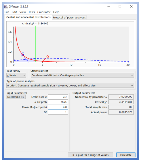
We can also use G*Power to calculate the sample size for the one-variable chi-square test. You need to select the screenshot of G*Power and detailed steps.
After typing all the numbers, you can hit the Calculate button. Then, you can see the sample size of 88, which is consistent with the output in method 1.

- Select “x2 tests” in Test family.
- Select “Goodness-of-fit tests: Contingency tables” in Statistical test.
- Select “A priori: Compute required sample size – given alpha, power, and effect size” in Type of power analysis.
- Type 0.3 in Effect size W.
- Type 0.05 in alpha err prob.
- Type 0.8 in power (1-beta err prob).
- Type 1 in Df.
Discussion