Chi Square Analysis in SPSS
Chi Square analysis (more specifically, Chi square independence test in this tutorial) is a statistical test used to determine if there is a significant association between two categorical variables. It assesses whether the observed frequencies of the variables in a contingency table differ significantly from the expected frequencies under the assumption of independence.
SPSS Data Example for Chi Square Analsysis
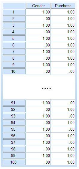
This hypothetical data set has two variables, gender (0 = Male vs. 1 = Female) and Purchase (0 = Not buying vs. 1 = Buying). The basic research question is to understand if men and women differ in terms of their intention to purchase a certain product. You can downloan this data set here via GitHub.
Null and Alternative Hypotheses
The following shows the null and alternative hypotheses for the chi square analysis (independence test in this tutorial).
- H0: There is no association between the two variables, and any observed differences are due to random chance.
- Ha: There is an association between the two variables.
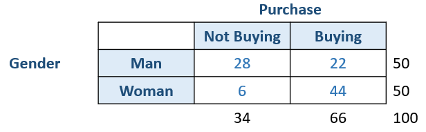
For instance, you want to test if women and men differ in terms of purchasing products from a certain brand. There are 50 men and 50 women in the data set. Among those 50 men, 22 do buy the product. In contrast, among 50 women, 44 of them buy the product.
Thus, we can actually write the null and alternative hypotheses for this example.
- H0: There is no association between gender and the purchase of the product.
- Ha: There is an association between gender and the purchase of the product.
Manual Calculation for Chi Square Analysis
The following is the main formula to calculate the chi-square independent test. O represents Observed Values, whereas E represents Expected Values based on the null hypothesis.
\( \chi^2 =\sum \frac{(O-E)^2}{E} \)
The following is the 2 by 2 contingency table with observed values and expected values.
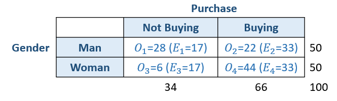
\( E_1 = \frac{34 \times 50}{100} = 17\)
\( E_2 = \frac{66 \times 50}{100} = 33\)
Thus, we can calculate the chi-square value as follows.
\( \chi^2 =\sum \frac{(O-E)^2}{E} = \frac{(28-17)^2}{17} + \frac{(22-33)^2}{33}+\frac{(6-17)^2}{17}+\frac{(44-33)^2}{33}= 21.57 \)
The degree of freedom for a 2 by 2 contingency table is 1. For the alpha value of 0.05, the critical chi-square value is 3.841. Thus, we can reject the null hypothesis and conclude that there is an association between gender and the purchase of the product.
If we examine the frequency counts closely, we can see that women are more likely to purchase that product than men (i.e., 44/50 vs. 22/50). The value of the chi-square test is to test that such frequency difference is statistically significantly different.
Steps of Doing Chi Square Analysis in SPSS
We are going to use the same data mentioned as an example above, namely the gender and purchase data. The following is a screenshot showing how it looks like in SPSS, including the first 10 and last 10 rows.
The following shows the steps of doing the chi-square independence test in SPSS.
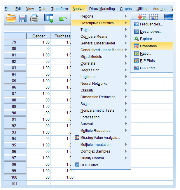
- Click Analyze > Descriptives Statistics > Crosstabs.
You will see the following window pops up after clicking Crosstabs.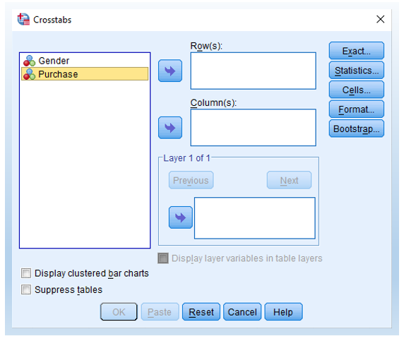
- Click Gender and then click the arrow to move it into Row(s): box. Do the same but move Purchase into the Column(s): box. After doing that, you will see the following.
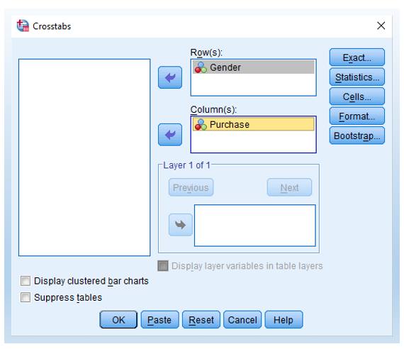
- Click Statistics. In the pop-up window, check Chi-square.
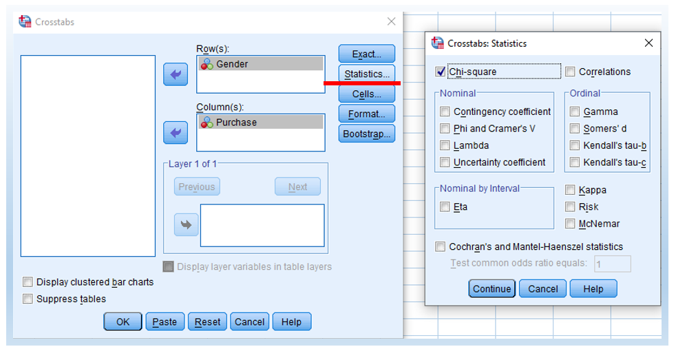
Then, click Continue in the pop-up window and OK in the main window. Then, you will see the following output.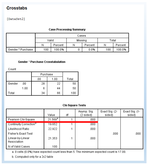
Result Interpretation and Report
We can see that the Pearson chi-square value is 21.57, which is consistent with our manual calculation earlier. Further, it also shows the degree of freedom (df) of 1. Finally, it shows the p-value (2-sided) of .000, which means the p-value is smaller than 0.001.
We can report the chi-square independent test as follows. In particular, we conducted a Pearson chi-square test and found that χ² = 21.57, p-value < .001. Thus, we reject the null hypothesis and conclude that there is an association between gender and the purchase of products. Further, based on the frequency count in the contingency table, we can conclude that women are significantly more likely to purchase the product than men (44/50 vs. 22/50).
Further Reading
You can watch the following YouTube video on Chi-square Analysis in SPSS. The video includes both Chi-square goodness-of-fit test and Chi-square test of independence in SPSS.
This tutorial is about the chi-square independence test in SPSS. Note that, in some situations, we might just want to focus on one variable to see if the distribution of different levels in the variable is even. For that case, it is called one variable chi-square test and you can click here to read more.
Further, the people in the 4 cells of the contingency table here are independent. That is, a person in one cell is different from another person in another cell. If there are repeated measures, we need to use McNemar’s Test, and you can click here to read more.
Finally, when one variable is a binary and it is a dependent variable, you can also use logistic regression. For instance, in the example above, you can also use logistic regression to test the relationship between gender and purchase intention. You can use purchase as DV and gender as IV and test the relationship in a logistic regression. In this case, the chi-square independence test and logistic regression are test the same thing. You can read my other tutorial on how to do logistic regression in SPSS.
Discussion