McNemar's Test in SPSS

This tutorial explains the definition of McNemar’s test, the writing of the null and alternative hypotheses for McNemar’s test, the steps of conducting it in SPSS, and how to interpret the output of McNemar’s test as well as how to report the results.

When to Use McNemar’s Test?

The McNemar test is used to analyze paired binary data to see if there is a significant difference in the distribution in terms of frequency counts of the two variables. Typically, these two variables measure the same thing, but at two different times (i.e., repeated measure).

When can you use McNemar’s test? If there are more than 2 variables or the variable has more than 2 levels, you can not use McNemar’s test. That is, McNemar’s test is for a 2 by 2 contingency table.

Further, McNemar’s test is used for repeated measures (i.e., paired data). That is, if these two variables are independent (i.e., measuring two different groups of objects or people), you can not use McNemar’s test either. Instead, you need to use a two-variable independent chi-square test.

Hypothesis and Test Statistic

Suppose that the measure happens at two different times and the measure has two outcomes, namely 1 and 2. The following is the table with 4 frequency counts.

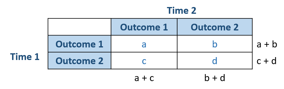
2 by 2 contingency table for McNemar's Test

The null hypothesis of McNemar’s test states that the marginal probabilities for two outcomes (i.e., Outcome 1 and Outcome 2) are the same, namely p_a + p_b = p_a + p_c and p_c + p_d = p_b + p_d.

Thus the null and alternative hypotheses are as follows.

H₀: p_b = p_c

H_a: p_b ≠ p_c

The test statistic formula for McNemar’s test is as follows.

\[ \chi^2 =\frac{(b-c)^2}{b+c} \]

Note that, in SPSS, the actual formula to calculate McNemar’s test is slightly different. It uses a continuity corrected version of McNemar’s test proposed by Edwards (see below).

\( \chi^2 =\frac{(b-c-1)^2}{b+c}\)

Data Example

Imagine that you ask 100 consumers if they would buy the product or not before the advertising (e.g., February). Then, after the advertising, they are asked again regarding their willingness to purchase the product (e.g., March). The research question is to understand if advertising makes an impact on their purchase intention.

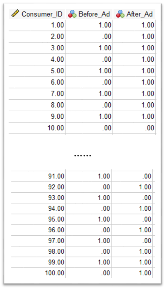
The following shows the first 10 rows and last 10 rows of data, out of 100 rows. There are 3 columns, consumer ID, Before Ad, and After Ad. In the data analysis, we do not need to use Consumer ID. Further, in Before Ad and After Ad, 1 represents that the consumer would like to purchase the product and 0 represents not.

Note that, this is a hypothetical data example. You can download the SPSS data file for McNemar’s test here. (Note that, if both columns are constant data, we can use a paired-sample t-test to do the data analysis.)

The data can also be summarized as a 2 by 2 contingency table as follows. It shows 4 cells of counts as well as row and column margins (totals).

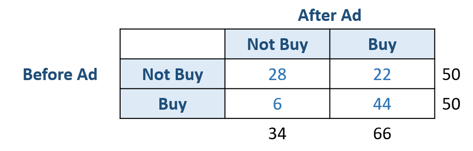
For this data, you can do a manual calculation as follows.

\( \chi^2 =\frac{(b-c-1)^2}{b+c} = \frac{(22-6-1)^2}{22+6} = 8.036\)

Steps of McNemar’s Test in SPSS

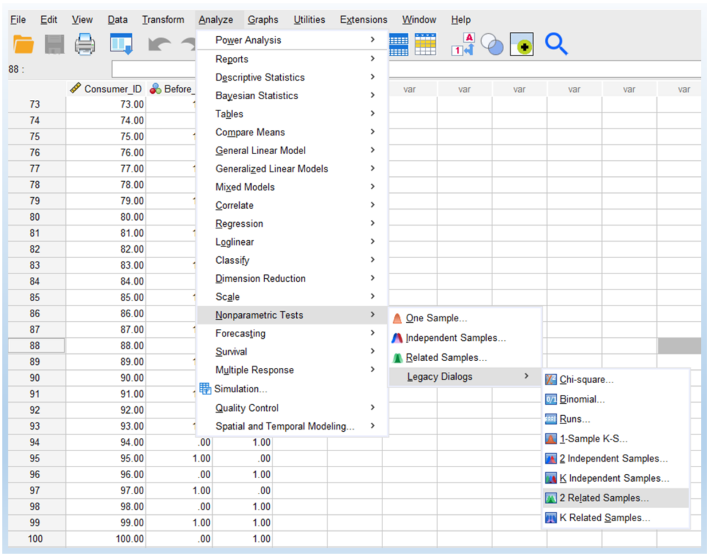
Click Analyze > Nonparametric Tests > Legacy Dialogs > 2 Related Samples…, as shown below.

You will then see the Two-Related-Samples Tests dialogue box shown below: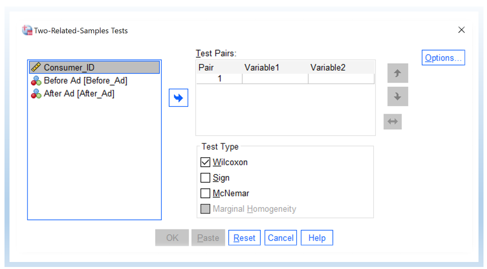
Transfer the variables of Before Ad and After Ad into the Test Pairs.

Next, uncheck Wilcoxon and check McNemar. Then, click OK.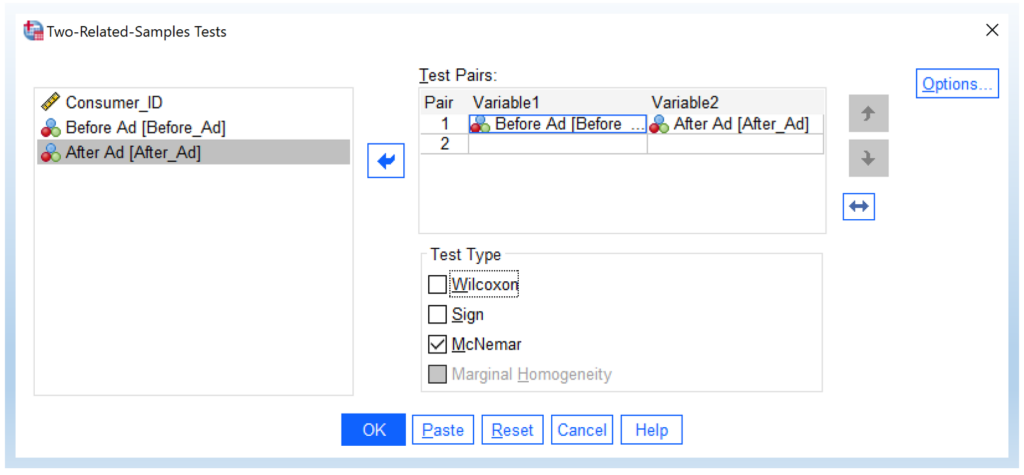

You will see the following output, which includes the 2 by 2 contingency table and the chi-square value of the McNemar test.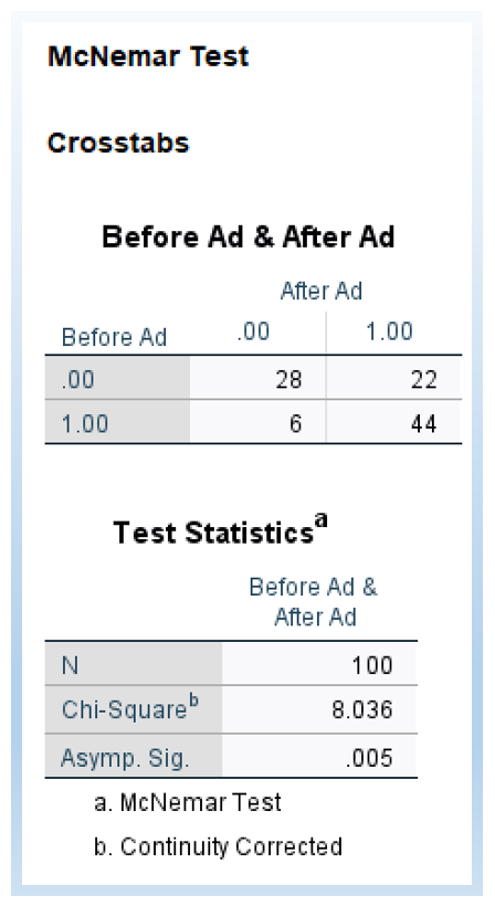

Result Interpretation

The McNemar test statistic follows a chi-square distribution with 1 degree of freedom. As shown above, the \( \chi^2 = 8.036\) and the p-value = 0.005.

Comparing the obtained p-value with the predetermined significance level (e.g., α = 0.05), we reject the null hypothesis and conclude that there is a significant difference between the two variables. In other words, advertising makes a difference in terms of impacting consumers’ purchase intentions.

In particular, before the advertising, buying and not buying are 50 and 50. After the advertising, the buying people are 66, and the not buying is 34. From the contingency table, we know that advertising makes a difference by increasing consumers’ purchase intention. Further, the McNemar test tells us that such a difference is statistically significant.

Report McNemar’s Test Result

After conducting the test, we need to write a report for McNemar’s test. The following is a write-up sample.

We conducted a McNemar test and obtained the following results: χ² = 8.036, p-value = 0.005. Based on these findings, we reject the null hypothesis, suggesting that the ratios of purchasing and not purchasing the product significantly differ between the periods before and after the advertising.

2 by 2 contingency table result for McNemar's test

Additionally, analyzing the count numbers in the 2×2 contingency table, we observed a rise in the number of individuals who purchased the product from 50 to 66, indicating that the advertising effectively increased people’s purchase intention.

McNemar’s Test in SPSS