Central Limit Theorem: Examples and Explanations
Central Limit Theorem (CLT) states that when you take a sufficiently large number of independent random samples from a population (regardless of the population’s original distribution), the sampling distribution of the sample mean will approach a normal distribution.
This tutorial uses two examples showing while the original data do not follow normal distribution (e.g., uniform distribution and binomial distribution), sample mean follows a normal distribution.
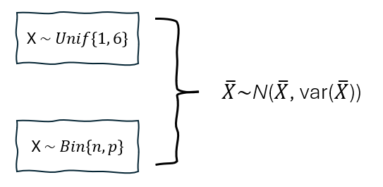
1. Rolling Dice (uniform distribution)
A fair 6-sided die has outcomes {1, 2, 3, 4, 5, 6}. Since it is a fair die, each number has a probability of 1/6=0.167. Thus, the distribution is uniform, not normal (see below).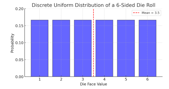
If we roll the die n times and take the average (i.e., x̄), the distribution of x̄ starts to resemble a normal distribution as n increases.
- Mean and Variance of \( X\)
Since X ~ Unif{1, 6}, the mean and variance of X are as follows.
\( \mu = \frac{1+6}{2} = 3.5\)
\( \sigma^2 = \frac{(1-3.5)^2 + (2-3.5)^2 + (3-3.5)^2 + (4-3.5)^2 + (5-3.5)^2 + (6-3.5)^2}{6} = \frac{17.5}{6} \approx 2.92 \) - Mean and Variance of \( \bar{X} \)
\( \mu_{\bar{X}} = 3.5\)
When n = 5: \( \sigma_{\bar{X}}^2= \frac{\sigma^2}{n} =\frac{\sigma^2}{5} =0.584\); \(\bar{X} \sim N(3.5, 0.584)\)
When n = 30: \( \sigma_{\bar{X}}^2= \frac{\sigma^2}{n} =\frac{\sigma^2}{30} =0.097\); \(\bar{X} \sim N(3.5, 0.097)\)
Further, from the formula of \( \bar{X} \) shown above, we can see that, the variance of \( \bar{X} \) will become smaller as \( n \) becomes larger. Thus, \( \bar{X} \) distribution has something to do with \( n\). - n times (rolls) per experiment
n is the size of sample in each draw. Increasing n (rolls per experiment) makes each sample mean more normally distributed (per CLT). Thus, setting n=30 (vs. n=5) makes the distribution of the mean gets narrower (and more normally distributed).
Visually, we can do it 100 times and calculate these 100 sample means. Using these 100 sample means, we can do a histogram plot. As we can see below, the histogram look like a normal distribution.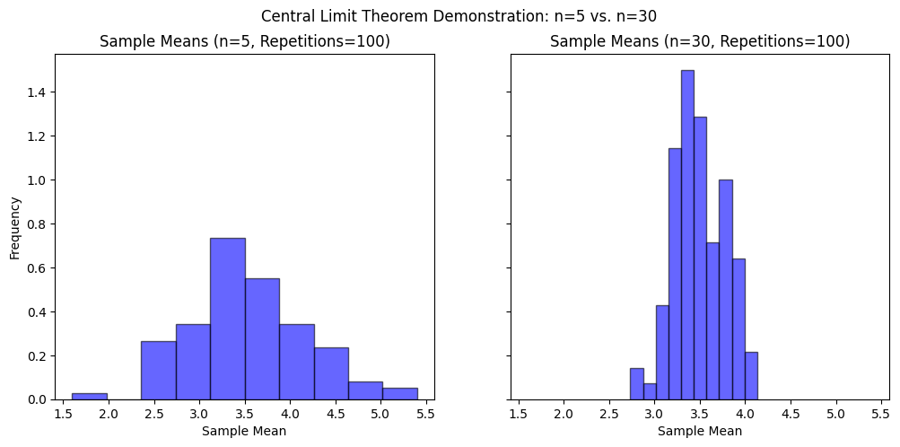
- Repetitions (e.g., 40 vs. 100)
Increasing repetitions (e.g., 40 vs. 100) improves visualization and makes the normality clearer but doesn’t change the underlying distribution. For instance, the following two figures (both n=30), one with repetitions = 40 and another one with repetitions = 100. As we can see that the repetitions = 100 visually more clearly follows normal distribution.
However, since n = 30 keeps the same, the underlying distribution is the same. Again, the distribution of \( \bar{X} \) has nothing to do with repetitions.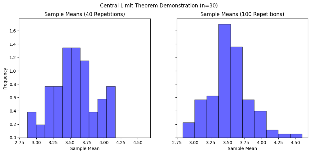
It is about the distribution of sample mean \( \bar{X} \).
2. What exactly is the difference between \( n \) and repetition?
As \( n \) increases, \( Var( \bar{X}) \) decreases. As we can see, the formula for \( \bar{X} \) involves \( n \) in variance, but no repetitions.
This means that sample means tend to cluster more tightly around the true mean as sample size grows (i.e., \(n\)). This is why the sampling distribution of the mean gets narrower with larger \( n \) , making it more reliable.
2. Conversation Rate (binomial distribution)
Suppose you want to calculate the click-through rate for an ad campaign (i.e., the percentage of people who view the ad and then click the advertising link). Since each ad view results in either a click (success) or no click (failure), and each view is independent of the others, the number of clicks in a sample (e.g., 100 visitors) follows a binomial distribution:
\( X \sim Bin(n,p) \)
- \( X \): Clicks observed in each sample.
- \( n\): the size of each sample.
- \( p \): true probability of a click.
- Mean and Variance \( X\)
\(\mu =np \)
\(\sigma^2=npq \)
For instance, if n=100 and p=5%, we can get \(\mu =np =100 \times 5 \%=5\);
\( \sigma^2=100 \times 5\% \times 95 \%=4.75\) - Mean and Variance \( \bar{X} \)
\( \bar{X} =\frac{X}{n}\)
\(E(\bar{X}) =\frac{E(X)}{n} =\frac{np}{n}=p\)
\(Var(\bar{X}) = \frac{Var(X)}{n^2}=\frac{npq}{n^2}=\frac{pq}{n}\)
Thus, \(\bar{X} \sim N(p, \frac{pq}{n}) \)
If \( p=5\% \) and \( n=100\), \(\bar{X} \sim N(p, \frac{pq}{n}) =N(5\%, 0.005) \)
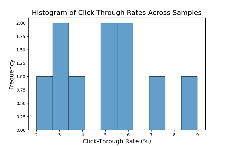
| Sample | X | n | \( \bar{X} \) | CTR |
|---|---|---|---|---|
| 1 | 4 | 100 | 4% | 4% |
| 2 | 9 | 100 | 9% | 9% |
| 3 | 6 | 100 | 6% | 6% |
| 4 | 5 | 100 | 5% | 5% |
| 5 | 3 | 100 | 3% | 3% |
| 6 | 3 | 100 | 3% | 3% |
| 7 | 2 | 100 | 2% | 2% |
| 8 | 7 | 100 | 7% | 7% |
| 9 | 5 | 100 | 5% | 5% |
| 10 | 6 | 100 | 6% | 6% |
We can do a histrogram of these 10 Click Through Rate (CTR). We can see that, it is kind of close to a normal distribution, but not very close.
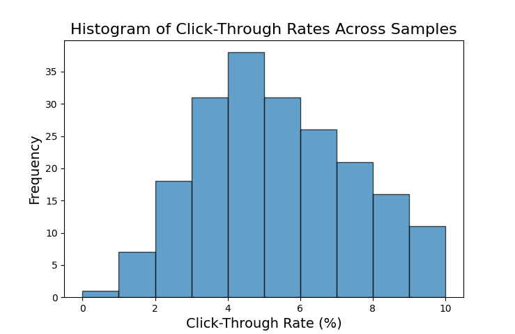
However, if we increase the frequency from 10 times to 200 times, each still with the sample size of 100, the figure will look more like a normal distribution. However, such increased repetitions only change the visual appeal, and do not change the underlying distribution of \( \bar{X} \), which is only impacted by \(n\) and not the number of the repetitions.
Key Takeaways:
- Individual Click Outcomes: Each person clicking or not follows a Bernoulli distribution (X∼Bern(p)).
- Total Clicks in a Sample: The number of successes in a sample of 100 follows a binomial distribution (X∼Bin(100,p)).
- Distribution of Sample Means: If we repeatedly take samples and compute CTRs, the sampling distribution of CTRs approximates a normal distribution.
Actually, in the example of click through rate, since it follows binomial distribution, the sample mean is exactly the click through rate. Thus, the histogram plot of CTR is actually the plot of sample mean, which follows a normal distribution. You can also refer to the table shown above, which helps you better understand the relationship between \(X\), \(n\), and \( \bar{X} \).
2. What exactly is sampling distribution of the sample mean?
The sampling distribution of the sample mean refers to the distribution of sample means when you repeatedly take random samples from a population and compute their means. For instance, both the distribution of 10 CTRs and the distribution of 200 CTRs are sampling distribution of the sample mean.
Discussion