Setup Hayes PROCESS in R (4 Steps)
The following shows steps of setup Hayes Mediation PROCESS in R.
- Click here to visit the offcial Hayes PROCESS R package webpage. Then, click “Download PROCESS v 4.3.”

- Open the downloaded zip file.
You should be able to find the folder of “PROCESS v4.3 for R.” Within the folder, you should be able to find the “process.R ” file.
 - Open “process.R”
Assuming that you can R Studio in your computer, you can double-click the process.R. R Studio will open the process.R as an independent R file tap. - Run “process.R”
The process.R code is very long. In order to select all its R code, right click the computer mouse and then click “Select all.” Then, hit Run in RStudio.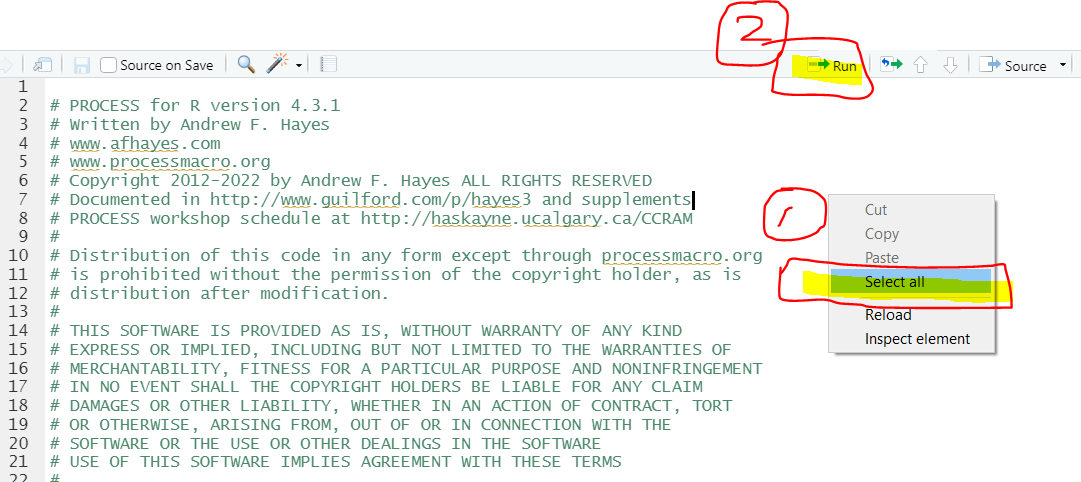
Then, the process() function is in the R environment (You will see the following output). That means that we can use the function.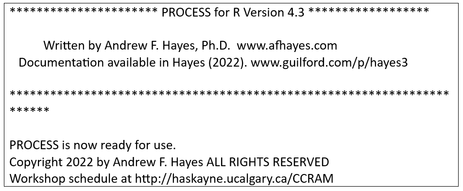
After setting up the PROCESS in R, we can use Model 4 as a simple example. In the following R code, we first download the data from GitHub. Then, run it using the process().
# Read data from GitHub
data_mediation <- read.csv("https://raw.githubusercontent.com/tidydatayt/mediation_analysis/main/mediation_hypothetical_data.csv")

# run model 4 using PROCESS in R as an example
process(data = data_mediation, y = "Y", x = "X", m ="M", model = 4)
After running the R code above, you should see the following output, which means that you setup PROCESS in R correctly. You can change variable names and the model number to do your own mediation analysis.
********************* PROCESS for R Version 4.3.1 *********************

           Written by Andrew F. Hayes, Ph.D.  www.afhayes.com
   Documentation available in Hayes (2022). www.guilford.com/p/hayes3

***********************************************************************

Model : 4
    Y : Y
    X : X
    M : M

Sample size: 100

Random seed: 611311


***********************************************************************
Outcome Variable: M

Model Summary:
          R      R-sq       MSE         F       df1
     0.2891    0.0836    1.2885    8.9359    1.0000
        df2         p
    98.0000    0.0035

Model:
             coeff        se         t         p
constant    0.6468    0.9247    0.6996    0.4859
X           0.0333    0.0111    2.9893    0.0035
              LLCI      ULCI
constant   -1.1881    2.4818
X           0.0112    0.0553

***********************************************************************
Outcome Variable: Y

Model Summary:
          R      R-sq       MSE         F       df1
     0.9566    0.9150    1.1382  522.3480    2.0000
        df2         p
    97.0000    0.0000

Model:
             coeff        se         t         p
constant    0.0327    0.8712    0.0376    0.9701
X           0.0023    0.0109    0.2093    0.8346
M           2.9318    0.0949   30.8807    0.0000
              LLCI      ULCI
constant   -1.6964    1.7618
X          -0.0194    0.0240
M           2.7433    3.1202

***********************************************************************
Bootstrapping progress:
  |>>>>>>>>>>>>>>>>>>>>>>>>>>>>>>>>>>>>>>>>>>>>>>>>>>>>>>>>>>>>>>| 100%

**************** DIRECT AND INDIRECT EFFECTS OF X ON Y ****************

Direct effect of X on Y:
     effect        se         t         p      LLCI      ULCI
     0.0023    0.0109    0.2093    0.8346   -0.0194    0.0240

Indirect effect(s) of X on Y:
     Effect    BootSE  BootLLCI  BootULCI
M    0.0975    0.0304    0.0368    0.1562

******************** ANALYSIS NOTES AND ERRORS ************************

Level of confidence for all confidence intervals in output: 95

Number of bootstraps for percentile bootstrap confidence intervals: 5000
Discussion