Two-Way ANOVA: Formulas and Calculation by Hand

This tutorial will first show the formulas for Two-way ANOVA and then use an example to show how you can calculate two-way ANOVA by hand.

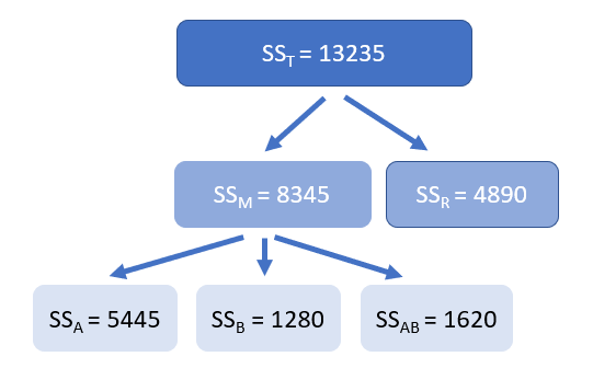
The following depicts the conceptual framework of the variance breaking down for two-way ANOVA. Typically, Two-way is used for experiment data analyses.

• SS_T is total variability.
• SS_M is variance explained by the experiment.
• SS_R is the unexplained variability.
• SS_A is variance explained by factor A.
• SS_B is variance explained by factor B.
• SS_AB is variance explained by the interaction of A and B.

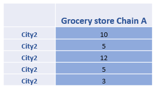
Data example for two-way ANOVA

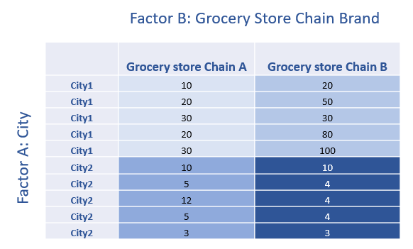
This is the data example for two-way ANOVA used in this tutorial. In particular, suppose you design an experiment to see how different cities and different grocery chain brands can impact sales. The following is the data. Thus, Factor A is City, and Factor B is Chain Brand.

Formula of total sums of squares (SS_T)

Suppose that we have factors A and B. Thus, the grand sum of squares SS_T can be written as follows.

SS_T=SS_M+SS_R = SS_A+ SS_B+SS_AB +SS_R

For SS_T, you can use the following formula.

\( SS_T=\sum \sum (x_{ij}-\bar{x})^2 \)

For the data example mentioned earlier, the grand mean is 22.5, and thus we can calculate the SS_T =13235.

SS_T=(10-22.5)²+(20-22.5)²+(20-22.5)²+…+(3-22.5)²= 13235

Formula of sum of squares (SS_M)

The next step is to calculate sum of squares (SS_M) for the whole model, namely the experiment model. The following is the formula for SS_M. We assume all the number of observations is the same across cells.

\[SS_{M}=n_{cell} \sum \sum (\bar{x_{ij}} -\bar{x})^2\]

We can use the formula above to calculate SS_M for the example mentioned earlier. Note that, we got 4 cells in the experiment, and each cell has 5 members.

SS_M=5(22-22.5)²+5(56-22.5)²+5(7-22.5)²+5(5-22.5)²=8345

The degree of freedom for SS_M is the number of cells minus 1. We have 4 cells, and thus, the degree of freedom is 3.

Formula of main effect of factor A(City)

We can then calculate the main effect of SS_A based on the following formula.

\[ SS_A= \sum n_i (\bar{x_i} -\bar{x})^2 \]

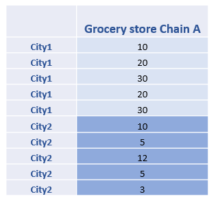
We can then calculate the sub-grand means for City 1, which is 39. Similarly, we can get the sub-grand means for City 2, which is 6.

Thus, we can calculate the main effect of SS_A.

SS_A= 10(39-22.5)²+10(6-22.5)²=5445

The degree of freedom for SS_A is the number of groups used, k, minus 1. Here, we have 2 groups, namely City 1 and City 2. Thus, the degree of freedom for SS_A is 2-1=1.

Formula of main effect of factor B (Chain Brand)

Similarly to factor A, we can calculate the SS_B as follows. The following is the formula.

\[ SS_B= \sum n_j (\bar{x_j} -\bar{x})^2 \]

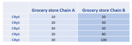
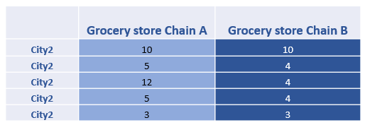
First, let’s show the data for Chain A and Chain B separately. We can get a sub-grand mean for Chain A is 14.5, and the sub-grand mean for Chain B is 30.5.

Then, similar to SS_A, we can calculate SS_B as follows.

SS_A= 10(14.5-22.5)²+10(30.5-22.5)²=1280

The degree of freedom for SS_B is also 2-1=1.

Two methods to calculate interaction effect SS_AB

Method 1

We can calculate the interaction effect of SS_AB using the following formula.

SS_AB =SS_M – SS_A– SS_B

Thus, we can get the SS_AB as 1620.

SS_AB =8345 – 5445- 1280 =1620

The degree of freedom for SS_AB is calculated as follows. Thus, the degree of freedom for SS_AB is 1.

df_AB=df_M-df_A-df_B=3-1-1=1

Method 2

There is another way to calculate SS_AB. The following is the formula, assuming the equal size of all cells, i.e., m.

\[ SS_{AB} = n_{cell} \sum \sum (\bar{x_{ij}}-\bar{x_i}-\bar{x_j}+\bar{x})^2 \]

Thus, we can calculate as follows. We can see that this method reaches the same result as the first method.

SS_AB= 5((22-14.5-39+22.5)²+(7-14.5-6+22.5)²+(56-30.5-6+22.5)²+(5-30.5-6+22.5)²)=1620

Calculation of residual sum of squares SS_R

We can also calculate SS_R using the following formula.

SS_R =SS²_{cell 1} + SS²_{cell 2}+…+SS²_{cell n}

The followings are Cell 1 and Cell 2 data. Cell 1’s mean is 22, whereas Cell 2’s mean is 7.

Thus, we can calculate the Sum of Squares for these two cells as follows.

SS²_cell1 =(10-22)²+2(20-22)²+2(30-22)²=280

SS²_cell2 =(10-7)²+2(5-7)²+(12-7)²+(3-7)²=58

Similarly, we can also calculate cell 3 and cell 4. The data is as follows.

SS²_cell3=(20-56)²+(50-56)²+(30-56)²+(80-56)²+(100-56)²=4520

SS²_cell4 =(10-5)²+3(4-5)²+(3-5)²=32

We can then calculate the SS_R, which is 4890.

SS_R =280+58+4520+32= 4890

We can check to see if our calculation so far is correct (see the updated variance breaking down figure shown below). As we can see, \( SS_T =13235 \) is based on the first calculation in this tutorial. At the same time, \( SS_M+SS_R\) also reach \(13235 \). Thus, we can see that our calculations are correct.

SS_T =SS_M+SS_R= 4890+8345 = 13235

The degree of freedom for SS_R is the number of observations minus the number of cells. Thus, it is 20-4=16.

Mean squares for two-way ANOVA

We can then calculate the mean squares for two-way ANOVA. Mean squares are the ratio of the sum of squares and the degree of freedom. The followings are the formulas and examples for mean squares of main effects, interaction effect, and residual in two-way ANOVA.

\[ MS_A=\frac{SS_A}{df_A} = \frac{5445}{1}=5445 \]

\[ MS_B=\frac{SS_B}{df_B} = \frac{1280}{1}=1280 \]

\[ MS_{AB}=\frac{SS_{AB}}{df_{AB}} = \frac{1620 }{1}=1620 \]

\[ MS_R=\frac{SS_R}{df_R} = \frac{4890}{16}=305.625 \]

F-ratio for two-way ANOVA

We can then calculate the F-ratio for two-way ANOVA as follows. That is, F-ratio is the ratio between the mean squares of that effect and the mean squares of residuals. We can see that the F-ratio for factor A is 17.816. The F-ratio for factor B is 4.188. The F-ratio for the interaction effect is 5.301.

\[ F_A=\frac{MS_A}{MS_R} = \frac{5445}{305.625}=17.816 \]

\[ F_B=\frac{MS_B}{MS_R} = \frac{1280}{305.625}=4.188 \]

\[ F_{AB}=\frac{MS_{AB}}{MS_R} = \frac{1620}{305.625}=5.301 \]

You can compare the results of this manual calculation of two-way ANOVA with the one using Excel shown in another tutorial (the link here). We can see the F-ratios are exactly the same. That means we calculate correctly here.