Understanding Interaction Effects in Data Analysis
This tutorial introduces the basic idea of interaction effects in data analysis. This tutorial includes what an interaction effect is, example of an interaction effect, and the statistical methods to do the analysis.
1. What are interaction effects? (The definition)
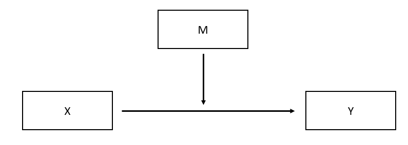
An interaction effect is when the effect of one variable (e.g., X) on another variable (e.g., Y) is dependent on a third variable (e.g., Y). The following is the visual illustration.
Y=β0+β1X+β2M+β3X×M
2. Example of Interaction Effects
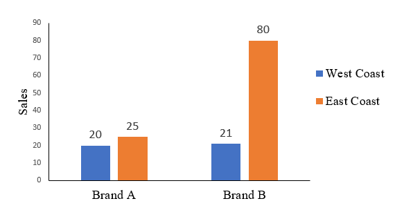
Suppose that you would like to how Brand A and Brand B are different in Sales. Thus, Brand (Brand A and Brand B) is the X, and Sales are the Y.
You calculate and find that Brand A has $45M sales and Brand B has $101M sales. Thus, you see the difference in sales. (Such difference can be called an effect.) Thus, the starting model looks like as follows.
Sales=β0+β1Brand
However, you realize that there is another variable (i.e., Region) that you need to consider such as West Coast and East Coast. Thus, the basic model can be expanded as follows.
Sales=β0+β1Brand+β2Region+β3Brand×Region
In particular, the difference between Brand A and Brand B occurs mainly on East Coast (25M vs. 80M). In contrast, the sales numbers on West Coast are roughly the same (20M vs. 21M).
Thus, you can see the importance of considering the third variable M, as it provides further insights into the basic effect of X on Y.
| East Coast | West Coast | ||
|---|---|---|---|
| Brand A | sales = 25M | sales = 20M | Brand A sales = 25+20=45M |
| Brand B | sales = 80M | sales = 21M | Brand B sales = 80+21=101M |
3. Statistical Methods to Analyze Interaction Effects
Depending on the different data types of X, M, and Y, you can have different ways to conduct the analysis to estimate β0, β1, β2, and β3.
Y=β0+β1X+β2M+β3X×M
The following table summarizes different statistical methods to estimate those coefficients.
| Y | X | M | Statistical Methods |
|---|---|---|---|
| Continuous | Continuous | Continuous | Linear Regression |
| Continuous | Continuous | Categorical | Linear Regression |
| Continuous | Categorical | Continuous | Linear Regression |
| Continuous | Categorical | Categorical | ANOVA or Linear Regression |
| Categorical | Continuous or Categorical | Continuous or Categorical | Logistic regression |
4. Interaction of Two Categorical Independent Variables in SPSS
Here, we are going to use a simulated dataset of two categorical independent variables to demonstrate how to conduct interaction analysis in SPSS.
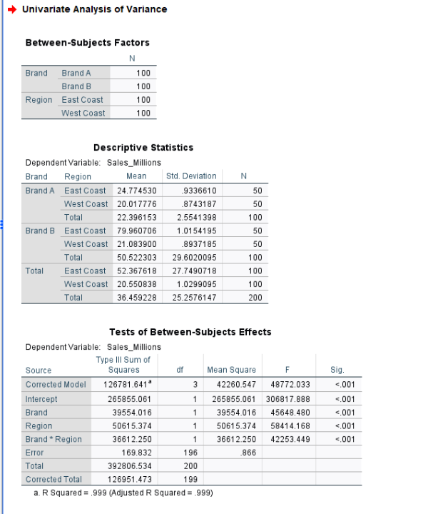
We can see that the interaction effect of Brand×Region has the p-value of < .001. This is smaller than 0.05. Thus, we reject the null hypothesis and conclude that the effect of Brand on Sales is moderated by Region.
Further Reading
I have provided tutorials to conduct such analysis in R, Python, and SPSS. The following shows a few examples.