Chi-Square Critical Value Table
Chi-Square Critical Value Table (Distribution Table)
| df | p = 0.995 | p = 0.99 | p = 0.975 | p = 0.95 | p = 0.9 | p = 0.75 | p = 0.5 | p = 0.25 | p = 0.1 | p = 0.05 | p = 0.025 | p = 0.01 | p = 0.005 |
|---|---|---|---|---|---|---|---|---|---|---|---|---|---|
| 1 | 0.000 | 0.000 | 0.001 | 0.004 | 0.016 | 0.102 | 0.455 | 1.323 | 2.706 | 3.841 | 5.024 | 6.635 | 7.879 |
| 2 | 0.010 | 0.020 | 0.051 | 0.103 | 0.211 | 0.575 | 1.386 | 2.773 | 4.605 | 5.991 | 7.378 | 9.210 | 10.597 |
| 3 | 0.072 | 0.115 | 0.216 | 0.352 | 0.584 | 1.213 | 2.366 | 4.108 | 6.251 | 7.815 | 9.348 | 11.345 | 12.838 |
| 4 | 0.207 | 0.297 | 0.484 | 0.711 | 1.064 | 1.923 | 3.357 | 5.385 | 7.779 | 9.488 | 11.143 | 13.277 | 14.860 |
| 5 | 0.412 | 0.554 | 0.831 | 1.145 | 1.610 | 2.675 | 4.351 | 6.626 | 9.236 | 11.070 | 12.833 | 15.086 | 16.750 |
| 6 | 0.676 | 0.872 | 1.237 | 1.635 | 2.204 | 3.455 | 5.348 | 7.841 | 10.645 | 12.592 | 14.449 | 16.812 | 18.548 |
| 7 | 0.989 | 1.239 | 1.690 | 2.167 | 2.833 | 4.255 | 6.346 | 9.037 | 12.017 | 14.067 | 16.013 | 18.475 | 20.278 |
| 8 | 1.344 | 1.646 | 2.180 | 2.733 | 3.490 | 5.071 | 7.344 | 10.219 | 13.362 | 15.507 | 17.535 | 20.090 | 21.955 |
| 9 | 1.735 | 2.088 | 2.700 | 3.325 | 4.168 | 5.899 | 8.343 | 11.389 | 14.684 | 16.919 | 19.023 | 21.666 | 23.589 |
| 10 | 2.156 | 2.558 | 3.247 | 3.940 | 4.865 | 6.737 | 9.342 | 12.549 | 15.987 | 18.307 | 20.483 | 23.209 | 25.188 |
| 11 | 2.603 | 3.053 | 3.816 | 4.575 | 5.578 | 7.584 | 10.341 | 13.701 | 17.275 | 19.675 | 21.920 | 24.725 | 26.757 |
| 12 | 3.074 | 3.571 | 4.404 | 5.226 | 6.304 | 8.438 | 11.340 | 14.845 | 18.549 | 21.026 | 23.337 | 26.217 | 28.300 |
| 13 | 3.565 | 4.107 | 5.009 | 5.892 | 7.042 | 9.299 | 12.340 | 15.984 | 19.812 | 22.362 | 24.736 | 27.688 | 29.819 |
| 14 | 4.075 | 4.660 | 5.629 | 6.571 | 7.790 | 10.165 | 13.339 | 17.117 | 21.064 | 23.685 | 26.119 | 29.141 | 31.319 |
| 15 | 4.601 | 5.229 | 6.262 | 7.261 | 8.547 | 11.037 | 14.339 | 18.245 | 22.307 | 24.996 | 27.488 | 30.578 | 32.801 |
| 16 | 5.142 | 5.812 | 6.908 | 7.962 | 9.312 | 11.912 | 15.338 | 19.369 | 23.542 | 26.296 | 28.845 | 32.000 | 34.267 |
| 17 | 5.697 | 6.408 | 7.564 | 8.672 | 10.085 | 12.792 | 16.338 | 20.489 | 24.769 | 27.587 | 30.191 | 33.409 | 35.718 |
| 18 | 6.265 | 7.015 | 8.231 | 9.390 | 10.865 | 13.675 | 17.338 | 21.605 | 25.989 | 28.869 | 31.526 | 34.805 | 37.156 |
| 19 | 6.844 | 7.633 | 8.907 | 10.117 | 11.651 | 14.562 | 18.338 | 22.718 | 27.204 | 30.144 | 32.852 | 36.191 | 38.582 |
| 20 | 7.434 | 8.260 | 9.591 | 10.851 | 12.443 | 15.452 | 19.337 | 23.828 | 28.412 | 31.410 | 34.170 | 37.566 | 39.997 |
| 21 | 8.034 | 8.897 | 10.283 | 11.591 | 13.240 | 16.344 | 20.337 | 24.935 | 29.615 | 32.671 | 35.479 | 38.932 | 41.401 |
| 22 | 8.643 | 9.542 | 10.982 | 12.338 | 14.041 | 17.240 | 21.337 | 26.039 | 30.813 | 33.924 | 36.781 | 40.289 | 42.796 |
| 23 | 9.260 | 10.196 | 11.689 | 13.091 | 14.848 | 18.137 | 22.337 | 27.141 | 32.007 | 35.172 | 38.076 | 41.638 | 44.181 |
| 24 | 9.886 | 10.856 | 12.401 | 13.848 | 15.659 | 19.037 | 23.337 | 28.241 | 33.196 | 36.415 | 39.364 | 42.980 | 45.559 |
| 25 | 10.520 | 11.524 | 13.120 | 14.611 | 16.473 | 19.939 | 24.337 | 29.339 | 34.382 | 37.652 | 40.646 | 44.314 | 46.928 |
| 26 | 11.160 | 12.198 | 13.844 | 15.379 | 17.292 | 20.843 | 25.336 | 30.435 | 35.563 | 38.885 | 41.923 | 45.642 | 48.290 |
| 27 | 11.808 | 12.879 | 14.573 | 16.151 | 18.114 | 21.749 | 26.336 | 31.528 | 36.741 | 40.113 | 43.195 | 46.963 | 49.645 |
| 28 | 12.461 | 13.565 | 15.308 | 16.928 | 18.939 | 22.657 | 27.336 | 32.620 | 37.916 | 41.337 | 44.461 | 48.278 | 50.993 |
| 29 | 13.121 | 14.256 | 16.047 | 17.708 | 19.768 | 23.567 | 28.336 | 33.711 | 39.087 | 42.557 | 45.722 | 49.588 | 52.336 |
| 30 | 13.787 | 14.953 | 16.791 | 18.493 | 20.599 | 24.478 | 29.336 | 34.800 | 40.256 | 43.773 | 46.979 | 50.892 | 53.672 |
| 40 | 20.707 | 22.164 | 24.433 | 26.509 | 29.051 | 33.660 | 39.335 | 45.616 | 51.805 | 55.758 | 59.342 | 63.691 | 66.766 |
| 50 | 27.991 | 29.707 | 32.357 | 34.764 | 37.689 | 42.942 | 49.335 | 56.334 | 63.167 | 67.505 | 71.420 | 76.154 | 79.490 |
| 60 | 35.534 | 37.485 | 40.482 | 43.188 | 46.459 | 52.294 | 59.335 | 66.981 | 74.397 | 79.082 | 83.298 | 88.379 | 91.952 |
| 70 | 43.275 | 45.442 | 48.758 | 51.739 | 55.329 | 61.698 | 69.334 | 77.577 | 85.527 | 90.531 | 95.023 | 100.425 | 104.215 |
| 80 | 51.172 | 53.540 | 57.153 | 60.391 | 64.278 | 71.145 | 79.334 | 88.130 | 96.578 | 101.879 | 106.629 | 112.329 | 116.321 |
| 90 | 59.196 | 61.754 | 65.647 | 69.126 | 73.291 | 80.625 | 89.334 | 98.650 | 107.565 | 113.145 | 118.136 | 124.116 | 128.299 |
| 100 | 67.328 | 70.065 | 74.222 | 77.929 | 82.358 | 90.133 | 99.334 | 109.141 | 118.498 | 124.342 | 129.561 | 135.807 | 140.169 |
Note: Values marked in bold represent common significance levels (α = 0.05 and α = 0.01)
- How can I locate the critical chi-square value from the table?
You can find the chi-square critical value based on degree of freedom (df) and the alpha level (shown as p-value on the table). For instance, if df=1 and alpha = 0.05, you can find the critical chi-square value of 3.841 (see the intersection of the two red boxes below in the figure). Typically, we go for p-value = 0.05 (i.e., the column of p-value = 0.05). You can choose other p-values if you have good reasons.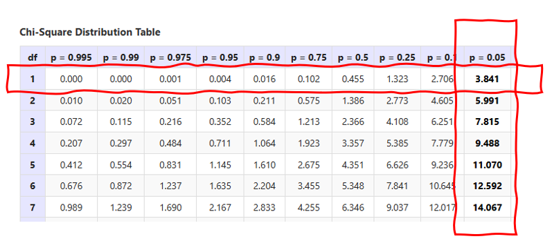
- What does a chi-square critcal value mean visually?
A critical chi-square value represents a threshold beyond which you would reject the null hypothesis in a chi-square test. It is determined based on the desired significance level (such as 0.05) and the degrees of freedom in your data. That is, if the chi-square value you calculate is greater than the critical value (falling in the critical region of orange color), you are going to reject the null hypothesis. For instance, if you get a calculated chi-square value of 4.2 (df = 1, p = 0.05), you are going to reject the null hypothesis.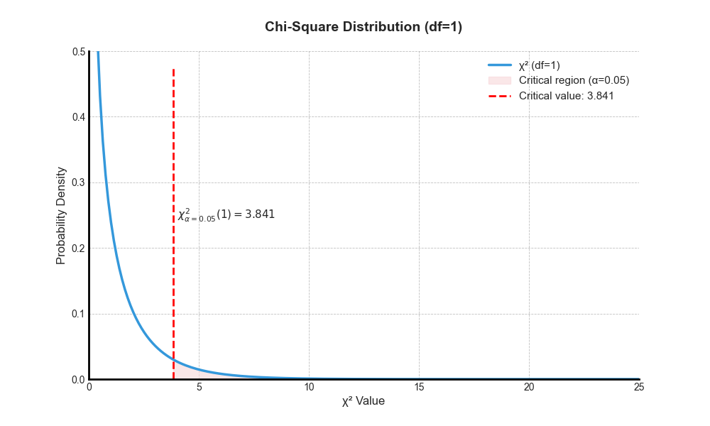
- Example of Chi-square test
For instance, you want to test if women and men differ in terms of purchasing products from a certain brand. There are 50 men and 50 women in the data set. Among those 50 men, 22 do buy the product. In contrast, among 50 women, 44 of them buy the product.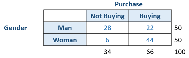
Thus, we can actually write the null and alternative hypotheses for this example.
H0: There is no association between gender and the purchase of the product.
Ha: There is an association between gender and the purchase of the product.
Then, you get the calculated chi-square value of 21.57 (click here to refer to the tutorial showing how to manually calculate the chi-square value). 21.57 is greater than the chi-square critical value of 3.841. Thus, we need to reject the the null hypothesis and conclude that there is an association between gender and the purchase of the product (i.e., Ha).
You can also refer to the figure below and see that 21.57 (green line) falls within the critical region, shown in orange. Thus, as long as the line falls within the critical region (i.e., to the right of the critical value line), we reject the null hypothesis.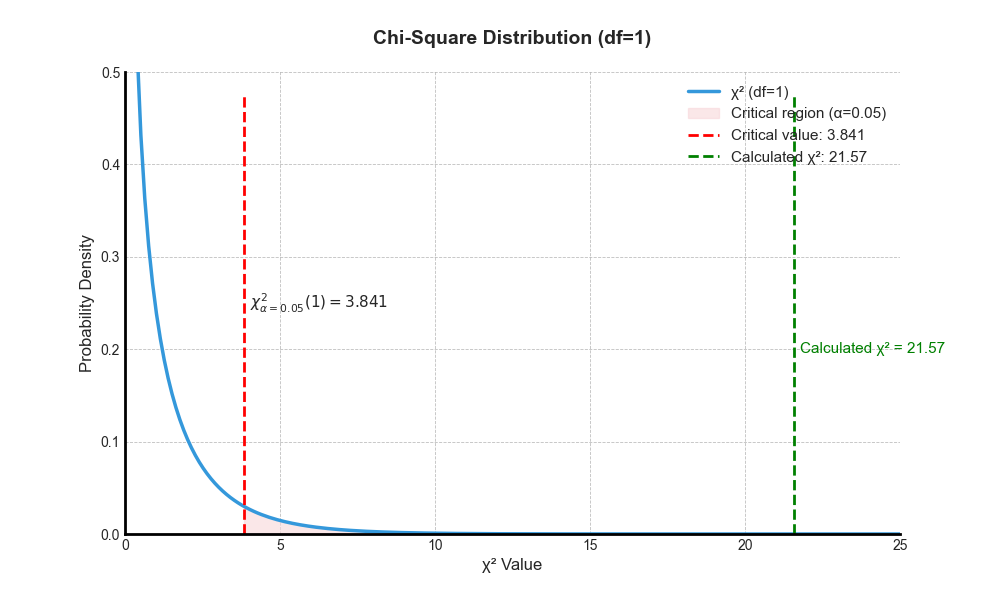
Additional Reding
You can learn more about chi-square test by referring to following tutorials:
Discussion