Johnson Neyman in SPSS (4 steps)
This tutorial explains what the Johnson Neyman technique is, when you can use the Johnson Neyman technique, and how you can do Johnson Neyman in SPSS.
What is the Johnson Neyman technique?
The Johnson Neyman technique is used for interaction effects with continuous variables as independent variables. In nature, it is a technique to help researchers and readers to understand linear regression with interaction effects. Thus, the Johnson Neyman technique is built on linear regression.
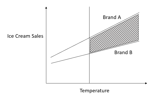
The Johnson Neyman technique is to find a cut-off point on one Moderator (i.e., M) where the effect of IV on the dependent variable (Y) is significant.
For instance, suppose IV Brand (Brand A and Brand B) has an effect on ice cream sales such that Brand A has higher sales than Brand B. But, the effect of Brand on sales is moderated by temperature. the Johnson Neyman technique is to help identify at what temperature Brand A and Brand B differ in sales.
When should you use the Johnson Neyman technique?
Johnson Neyman is typically used when (1) the dependent variable is a continuous variable and (2) the moderator is a continuous variable. (i.e., the situations of A and C in the following table)
Y=b0+b1X+b2M+b3X×M
| Situation | Y | X | M | statistical Methods |
|---|---|---|---|---|
| A | Continuous | Continuous | Continuous | Johnson Neyman on the top of Linear Regression |
| B | Continuous | Continuous | Categorical | Linear Regression |
| C | Continuous | Categorical | Continuous | Johnson Neyman on the top of Linear Regression |
| D | Continuous | Categorical | Categorical | ANOVA (no need for Johnson Neyman) |
Question 1: Can you use the Johnson Neyman technique when the moderator is a categorical variable and the X is a continuous variable (i.e., situation B in the table above)?
- The answer is yes since the framing of X and M is really based on your research question, rather than statistical technique. However, you should have a very clear idea of what you are actually doing.
Question 2: Can you use the Johnson Neyman technique when the categorical variable of X is more than 2 levels (i.e., beyond binary)?
- The answer is yes but it is beyond the discussion of this tutorial. You can refer to Amanda Kay Montoya’s master’s thesis.
Question 3: Can you use Johnson Neyman for situations when Y is a binary (i.e., for logistic regression)?
- The answer is yes again. But, this is beyond the discussion of this tutorial, and you can refer to Hayes and Matthes’s 2009 paper.
Data Preparation
Final Dataset being Used
You can also download an updated version of SPSS sav file posted here (GitHub Link ), where the variable of Gender_dummy has been added. Thus, you do not need to do the SPSS syntax by yourself.
Testing Model
The following is the model that we are going to test.
write = b0 + b1 socst + b2 Gender_Dummy + b3 socst *Gender_Dummy
| Variable name in SPSS | DV vs. IVs | data type | Meaning |
|---|---|---|---|
| write | DV | Continuous variable | writing scores |
| Gender_Dummy (female) | IV1 | Categorical variable | female, male |
| socst | IV2 | Continuous variable | test score for social studies |
Background of the Dataset
We are going to use the dataset called ![]() hsbdemo (click here to download), and this dataset has been used in some other tutorials online (See this UCLA webpage on the interaction between categorical and continuous variables). The following is the model that we are going to test.
hsbdemo (click here to download), and this dataset has been used in some other tutorials online (See this UCLA webpage on the interaction between categorical and continuous variables). The following is the model that we are going to test.
Note that, in the original dataset, there is no variable of Gender_Dummy. We need to create this variable using the following SPSS syntax.
* recoding female to be dummy coding in a new variable called Gender_dummy.
if female='female' Gender_dummy=1.    /* female
if female='male' Gender_dummy=0.    /* male
execute.
Steps of Johnson Neyman in SPSS
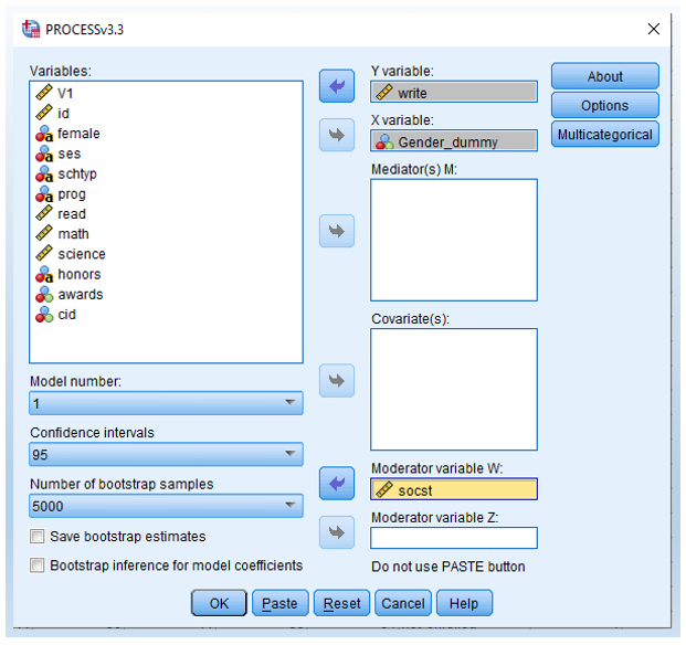
- Analyze > Regression > PROCESS by Andrew F. Hayes
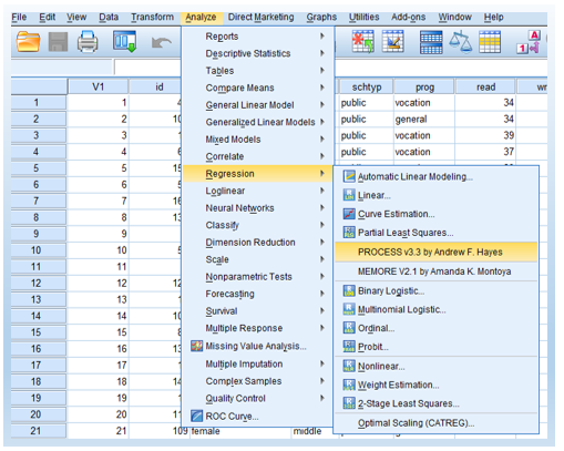
You will then see the following main PROCESS popup window.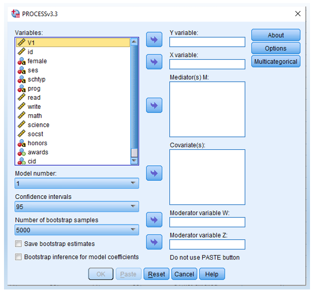
- Drag variables write as Y variable, Gender_dummy as X variable, and socst as Moderator Variable W.
- Click Options and check Generate code for visualizing interactions and Johnson-Neyman output.
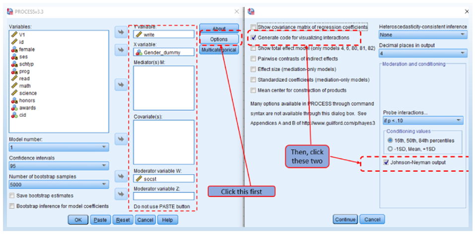
Then, click Continue in the secondary window and OK in the main window. You will then see the results showing up in the next section.
Output and interpretation of Johnson Neyman in SPSS
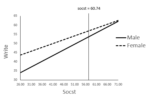
After clicking Continue and OK in step 3 discussed above, you will see the following output of Johnson Neyman in SPSS. As you can see that the interaction p-value is 0.0331, and thus the interaction of socst *Gender_Dummy is significant.
Further, we can see that the cut-off point is socst = 60.7426, where the p-value =0.05. Thus, it means that male and female students are significantly different in writing scores when socst < 60.7426. In contrast, when socst > 60.7426, male and female students are NOT significantly different in writing scores when socst < 60.7426.
Run MATRIX procedure:

*************** PROCESS Procedure for SPSS Version 3.3 *******************

          Written by Andrew F. Hayes, Ph.D.       www.afhayes.com
    Documentation available in Hayes (2018). www.guilford.com/p/hayes3

**************************************************************************
Model  : 1
    Y  : write
    X  : Gender_d
    W  : socst

Sample
Size:  200

**************************************************************************
OUTCOME VARIABLE:
 write

Model Summary
          R       R-sq        MSE          F        df1        df2          p
      .6556      .4299    52.0073    49.2587     3.0000   196.0000      .0000

Model
              coeff         se          t          p       LLCI       ULCI
constant    32.7619     3.6539     8.9662      .0000    25.5559    39.9680
Gender_d   -15.0000     5.0979    -2.9424      .0036   -25.0539    -4.9461
socst         .4201      .0678     6.1953      .0000      .2863      .5538
Int_1         .2047      .0954     2.1466      .0331      .0166      .3928

Product terms key:
 Int_1    :        Gender_d x        socst

Test(s) of highest order unconditional interaction(s):
       R2-chng          F        df1        df2          p
X*W      .0134     4.6080     1.0000   196.0000      .0331
----------
    Focal predict: Gender_d (X)
          Mod var: socst    (W)

Conditional effects of the focal predictor at values of the moderator(s):

      socst     Effect         se          t          p       LLCI       ULCI
    41.0000    -6.6061     1.4918    -4.4283      .0000    -9.5482    -3.6641
    52.0000    -4.3541     1.0260    -4.2437      .0000    -6.3776    -2.3307
    65.2000    -1.6517     1.5972    -1.0341      .3024    -4.8016     1.4982

Moderator value(s) defining Johnson-Neyman significance region(s):
      Value    % below    % above
    60.7426    67.5000    32.5000

Conditional effect of focal predictor at values of the moderator:
      socst     Effect         se          t          p       LLCI       ULCI
    26.0000    -9.6771     2.7152    -3.5641      .0005   -15.0317    -4.3224
    28.2500    -9.2164     2.5178    -3.6606      .0003   -14.1818    -4.2510
    30.5000    -8.7558     2.3234    -3.7685      .0002   -13.3379    -4.1737
    32.7500    -8.2951     2.1330    -3.8890      .0001   -12.5017    -4.0886
    35.0000    -7.8345     1.9475    -4.0228      .0001   -11.6753    -3.9937
    37.2500    -7.3739     1.7687    -4.1690      .0000   -10.8620    -3.8857
    39.5000    -6.9132     1.5987    -4.3242      .0000   -10.0661    -3.7603
    41.7500    -6.4526     1.4407    -4.4788      .0000    -9.2938    -3.6114
    44.0000    -5.9919     1.2990    -4.6129      .0000    -8.5537    -3.4302
    46.2500    -5.5313     1.1795    -4.6897      .0000    -7.8574    -3.2052
    48.5000    -5.0707     1.0895    -4.6540      .0000    -7.2194    -2.9219
    50.7500    -4.6100     1.0369    -4.4461      .0000    -6.6549    -2.5652
    53.0000    -4.1494     1.0273    -4.0393      .0001    -6.1753    -2.1235
    55.2500    -3.6887     1.0618    -3.4740      .0006    -5.7828    -1.5947
    57.5000    -3.2281     1.1366    -2.8402      .0050    -5.4696     -.9866
    59.7500    -2.7675     1.2443    -2.2242      .0273    -5.2213     -.3136
    60.7426    -2.5642     1.3002    -1.9721      .0500    -5.1285      .0000
    62.0000    -2.3068     1.3772    -1.6750      .0955    -5.0229      .4092
    64.2500    -1.8462     1.5288    -1.2076      .2287    -4.8613     1.1689
    66.5000    -1.3855     1.6941     -.8179      .4144    -4.7266     1.9555
    68.7500     -.9249     1.8695     -.4947      .6213    -4.6117     2.7619
    71.0000     -.4643     2.0523     -.2262      .8213    -4.5116     3.5831

Data for visualizing the conditional effect of the focal predictor:
Paste text below into a SPSS syntax window and execute to produce plot.

DATA LIST FREE/
   Gender_d   socst      write      .
BEGIN DATA.
      .0000    41.0000    49.9847
     1.0000    41.0000    43.3786
      .0000    52.0000    54.6054
     1.0000    52.0000    50.2513
      .0000    65.2000    60.1503
     1.0000    65.2000    58.4986
END DATA.
GRAPH/SCATTERPLOT=
 socst    WITH     write    BY       Gender_d .

*********************** ANALYSIS NOTES AND ERRORS ************************

Level of confidence for all confidence intervals in output:
  95.0000

W values in conditional tables are the 16th, 50th, and 84th percentiles.

NOTE: Variables names longer than eight characters can produce incorrect output.
      Shorter variable names are recommended.

------ END MATRIX -----
Optional Step 4: Plot Johnson Neyman in SPSS and Excel
Besides the 3 steps shown above, there is an optional step 4 to plot the Johnson Neyman in SPSS and Excel. That is, we can use the syntax generated by the output in step 3 to plot the interaction in SPSS.
DATA LIST FREE/
   Gender_d   socst      write      .
BEGIN DATA.
      .0000    41.0000    49.9847
     1.0000    41.0000    43.3786
      .0000    52.0000    54.6054
     1.0000    52.0000    50.2513
      .0000    65.2000    60.1503
     1.0000    65.2000    58.4986
END DATA.
GRAPH/SCATTERPLOT=
 socst    WITH     write    BY       Gender_d .
That is, we can run the syntax above in SPSS, and it will generate the plot below.
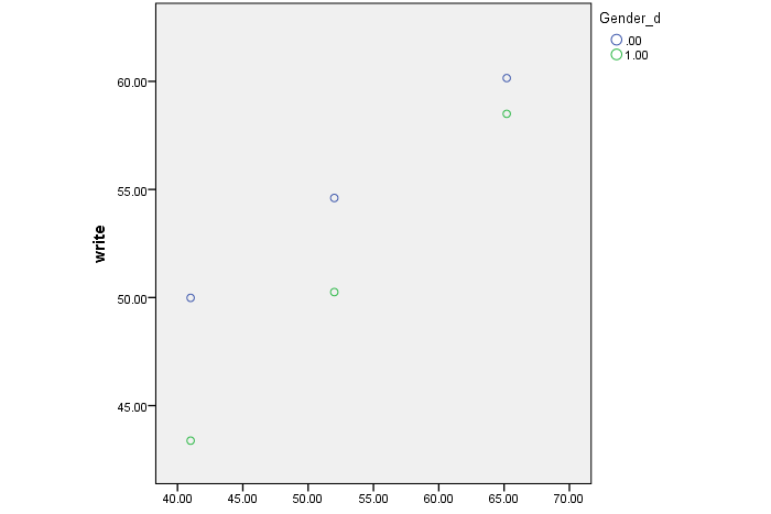
Note that, the plot from SPSS is a bit generic. In order to make it look better, we can use Excel. The following is the plot I did via Excel.
Further Reading
There are other resources to understand how to do Johnson Neyman in SPSS such as these two YouTube videos:
- One shows the exact steps of Johnson Neyman in SPSS.
- And another one show how to plot Johnson Neyman using Excel.
Discussion