One-Way ANOVA in Excel
This tutorial shows how you can do one-way ANOVA (analysis of variance) in Excel. Note that, one-way ANOVA is also called single factor ANOVA.
Steps of One-Way ANOVA in Excel
Step 1: Prepare the data
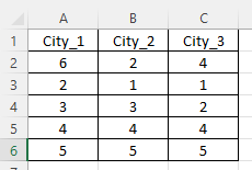
Suppose we would like to see whether 3 cities differ in terms of household size. We sample 5 households from each city. The following is the data for this analysis.
The null hypothesis and alternative hypothesis for one-way ANOVA are as follows.
- Null Hypothesis: All 3 cities have the same household size.
- Alternative Hypothesis: At least two cities does not have the same household size.
Step 2: Click “Data Analysis”
Next, click “Data” menu and find the “Analysis” box. Then, click “Data Analysis” module.

If you can not find the Data Analysis” module, please refer to another tutorial showing how to add “Data Analysis” to Excel.
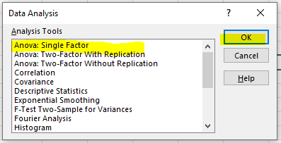
Step 3: Click “ANOVA: Single Factor”
On the pop-up window, click the “ANOVA: Single Factor” and then click “OK.”
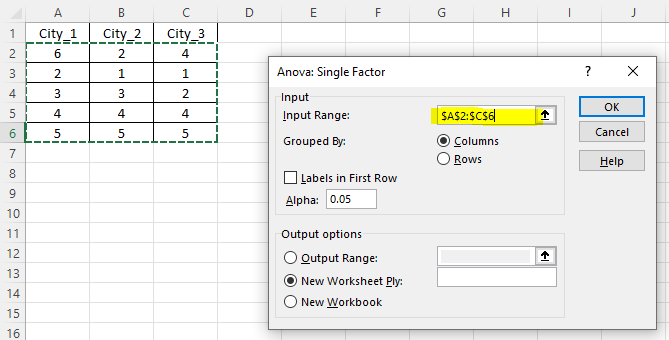
Step 4: Add input range
Select A2 to C6, namely all cells with data, in the “Input Range.” Then, click “OK.”
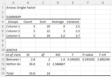
Step 5: Interpret the output
Since the p-value = 0.59, which is greater than 0.05, we fail to reject the null hypothesis. Thus, we can conclude that these 3 cities have roughly the same household size.
If you want to download this Excel file, you can click here to download it from GitHub.