Linear Regression in Excel
This tutorial shows how you can do linear regression in Excel with examples and detailed steps.
Steps of Linear Regression in Excel
Step 1: Prepare data and hypothesis
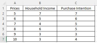
We want to test how consumer purchase intention can be impacted by price as well as by household income. Thus, consumer purchase intention is the Y, whereas price and household income are the Xs.
Step 2: Click “Data Analysis”
Next, click the “Data” menu and find the “Analysis” box. Then, click the “Data Analysis” module.
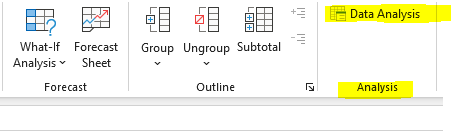
If you can not find the Data Analysis” module, please refer to another tutorial showing how to fix that.
Step 3: Click “Regression”
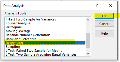
Click “Regression” and then “OK.”
Step 4: Define input ranges in Excel
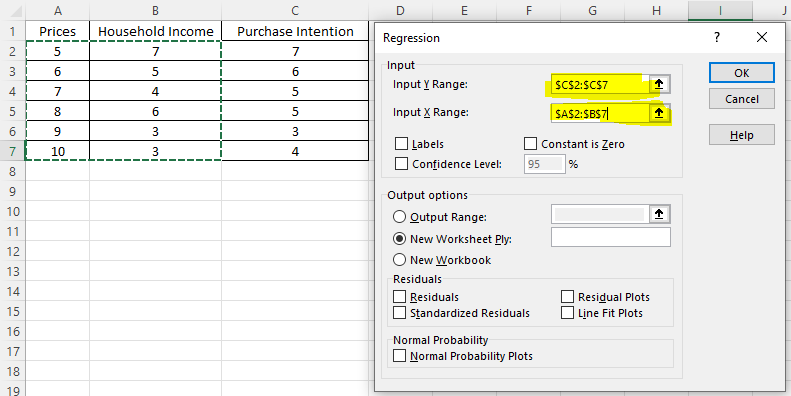
Select C2 to C7 into “Input Y Range” and A2 to B7 into “Input X Range.” Then click “OK.”
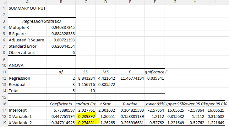
Step 5: Interpret Excel output
We can see 𝑏₀ = 6.73, 𝑏₁ = -0.45, and b2 =0.35. We can write the estimated regression function below. However, note that all the p-value for both Xs (i.e., 0.2398 and 0.2748) are greater than 0.05, and thus these two predictors, price and household income, are not statistically significant.
Purchage Intention=6.73−0.45Price+0.35Household Income
If you want to download this Excel file, you can click here to download it from GitHub.