Orthogonal Projection
This tutorial explains what an orthogonal projection is in linear algebra. Further, it provides proof that the difference between a vector and a subspace is orthogonal to that subspace.
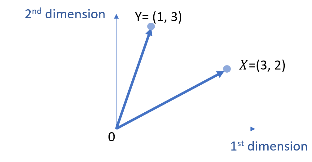
Let’s define two vectors, \(\vec{X} \) and \(\vec{Y} \), and we want to find the shortest distance between \(\vec{Y} \) and the subspace defined by the span of \(\vec{X} \).
To simplify the discussion, we use the 2-dimensional space for visualization.
\( \vec{X}=\left[\begin{array}{ccc}
3\\
2 \end{array}
\right]\)
\( \vec{Y}=\left[\begin{array}{ccc}
1\\
3 \end{array}
\right]\)
Further, we name \( L \) the subspace defined by the span of the vector \(\vec{X} \). The projection of \(\vec{Y} \) → onto \( L \) is the closest point on \( L \) to \(\vec{Y} \).
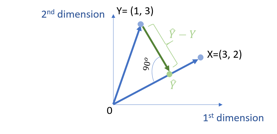
Intuitively, the shortest distance between these two points is orthogonal to the space \( L \). The proof is provided in the next section.
\( ( \hat{Y}-\vec{Y} ) \cdot \vec{X} = 0 \)
\( ( c \vec{X}-\vec{Y} ) \cdot \vec{X} = 0 \)
We can further get the following:
\( c \vec{X} \cdot \vec{X} – \vec{Y} \cdot \vec{X}= 0 \)
Further,
\( c = \frac{\vec{Y} \cdot \vec{X}}{\vec{X} \cdot \vec{X}} \)
Note that, the doct product \( \cdot \) means that \( \vec{X} \cdot \vec{Y} =x_1*y_1+…+ x_n*y_n \).
Proof
This section provides proof that the shortest distance between a point and a space is that the line connecting the point and the space is orthogonal to that space.
In particular, since \( \hat{Y} =c X \), we know that \( \hat{Y} \) is on space of \( L \). However, we do not know the exact location of \( \hat{Y} \). To determine the location of \( \hat{Y} \), it is to equivalently determine the value of c.
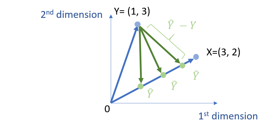
And, we target the make the difference between \( Y \) and \( \hat{Y} \) is minimal. Thus,
min | \( \hat{Y} – Y \)|
We can then just use the Euclidean distance to measure it. Thus, we can get the following.
min \( \sqrt{ \sum_{i} (\hat{Y_i} -Y_{i})^2 } =\sqrt{ \sum_{i} ( cX_{i} – Y_{i} )^2 } \)
Given the monotonicity, we can remove the square root notation and get the following.
min \( \sum_i (cX_{i} – Y_{i} )^2 \)
The function above has a quadratic with respect to c, and thus it has the minimum value when calculating the first-order derivative.
\( \frac{d}{dc} \sum_i (cX_{i}-Y_{i})^2 =0 \)
We can thus get the following.
\( \begin{align} \frac{d}{dc} \sum_i (cX_{i}-Y_{i})^2 &= \sum_i 2 X_{i} (cX_{i}-Y_{i}) \\ &=2 \sum_i X_{i} (cX_{i}-Y_{i}) \\ &= 2 \sum_i ( cX_{i} X_{i}-X_{i}Y_{i}) \end{align} \)
Thus, we can further get the following.
\( 2 \sum_i ( cX_{i} X_{i}-X_{i}Y_{i}) =0 \)
Thus, we remove the \( \sum \) notation by using vector dot product format.
\( cX^{T} \cdot X -X^T \cdot Y =0 \) [eq. 1]
Based on eq. 1, we can get eq. 2, which means that the vector of \( \hat{Y} – Y \) is orthogonal to the space of \( L\), which is defined by the vector of X. That is, the vector \( Y – \hat{Y} \) and \( L\) are perpendicular to each other (i.e., 90 degrees).
\( X^{T} \cdot (c X-Y) =0 \)
\( X^{T} \cdot (\hat{Y}-Y) =0 \) [eq. 2]
Further, from eq. 1, we can also get the value of c.
\( c= (X^{T} \cdot X)^{-1} \cdot X^{T} \cdot Y \)
Thus,
\( \hat{Y}=c X= X c = X \cdot (X^{T} \cdot X)^{-1} \cdot X^{T} \cdot Y = P \cdot Y \)
where,
\( P = X \cdot (X^{T} \cdot X)^{-1} \cdot X^{T} \)
Note that, P is a square matrix, and you can easily prove the following two properties of P.
\( P^2 = P \)
\( P^T = P \)
Thus, P is an orthogonal projection matrix (Wikipedia) since P2 = p = pT. Thus, this tutorial provides proof that the shortest distance between a vector arrow point and a subspace is through a line that is orthogonal to that subspace.
Discussion