Linear Regression and Orthogonal Projection
This tutorial explains why and how linear regression can be viewed as an orthogonal projection on 2 and 3-dimensional spaces.
Projection with 2 Dimensions
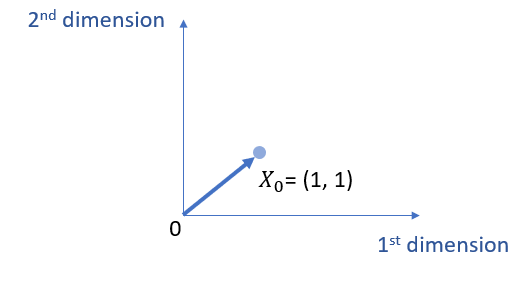
Suppose that both X0 and Y have 2 dimensions (e.g., 2 observations from 2 participants). It is worth pointing out that, when talking about dimensions here, we refer to the number of observations (i.e., rows in a matrix format), rather than the number of independent variables (i.e., columns in a matrix, i.e., Xs).1
Relatedly, I purposely use X0 (rather than X or X1) because I want to emphasize that we are talking about one X variable here and this X variable (i.e., X0) is an all 1’s vector (i.e., the intercept, constant).
\( X_0 =\left[\begin{array}{ccc}
1 \\
1 \end{array}
\right]\)
That is, here, we are actually just estimating the regression coefficient of b0, without even estimating b1, i.e., the slope. The main reason for such simplicity is that, if there is another column of data (e.g., X1), and we need to estimate b1, namely the slope, we then do not have enough degree of freedom. (Note that, 2 observations give us only 2 degrees of freedom to use.)
\( Y = b_0 X_0 \)
Thus, by replacing X0 with the actual all 1’s vector, we can get the following.
\( Y = b_0 \left[\begin{array}{ccc}
1 \\
1 \end{array}
\right] \)
Further, the discussion here limits X0 to 2 dimensions space (e.g., 2 observations), which is easier to plot and understand on a computer screen, i.e., the screen you see now. We can then draw a figure as follows.
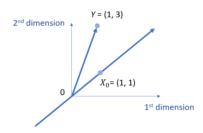
Suppose that we have 2 observations for Y as well.
\( Y =\left[\begin{array}{ccc}
1\\
3 \end{array}
\right]\)
We can then add Y into the same plane, as well as expand X0 as a span subspace.
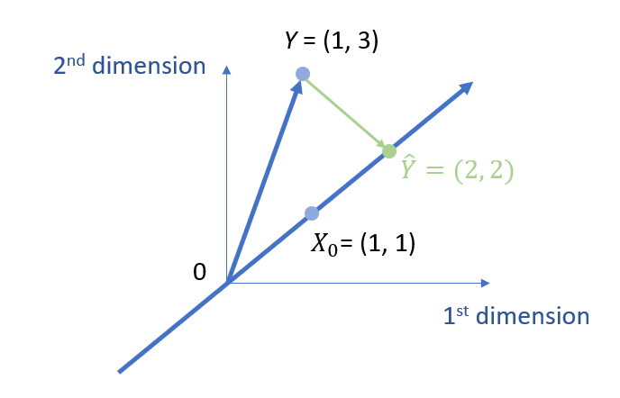
Here, the finding of b0 needs to meet two requirements:
- (1) we are finding the value b0 on the subspace defined by the span of vector X0;
- (2) based on the basic idea of linear regression, we want to make sure the residuals are the minimal.
As discussed in my other tutorial on orthogonal projection, these two requirements will lead to finding an orthogonal projection on the subspace.
Further, based on my other tutorial on mean as a projection, we know that b0 actually is the mean of all the dimensions in Y, namely,
\( b_0 = \frac{1+3}{2} = 2 \)
We can show the value of b0 visually as follows.
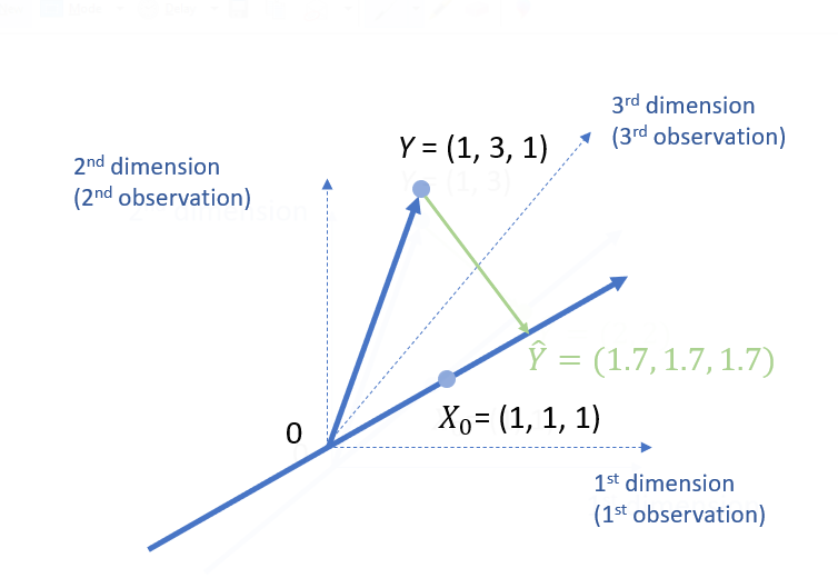
Projection with 3 Dimensions
This section explains what it means to have 3 dimensions in the context of linear regression and orthogonal projection.
For 3 dimensions, we can still just calculate the mean for Y, if you only have an all 1’s vector X0.
\( Y =\left[\begin{array}{ccc}
1\\
3 \\ 1 \end{array}
\right]; X =\left[\begin{array}{ccc}
1 \\
1 \\ 1 \end{array}
\right]\)
\( Y = b_0 X_0 \)
As we know, basically, b0 is the mean of all the dimensions in Y.
\( b_0 = \frac{1+3+1}{3} = 1.7 \)
Since we have 3 dimensions (i.e., 3 observations), it allows us to estimate another parameter such as the slope, i.e., b1. The following is the data.
\( Y =\left[\begin{array}{ccc}
1\\
3 \\ 1 \end{array}
\right]; X =\left[\begin{array}{ccc}
1 & 2\\
1 & 3 \\ 1 & 3 \end{array}
\right]\)
For this, we are going to need to estimate both b0 and b1.
\( Y = b_0 X_0 +b_1 X_1 \)
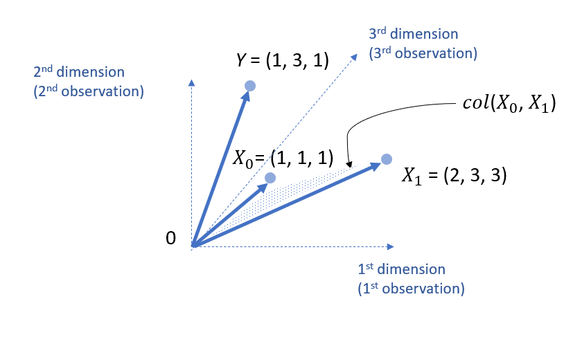
For this data set, we can add X1 into the 3 dimension space.

Note that, X1 and X0 define a column space, col (X0, X1).
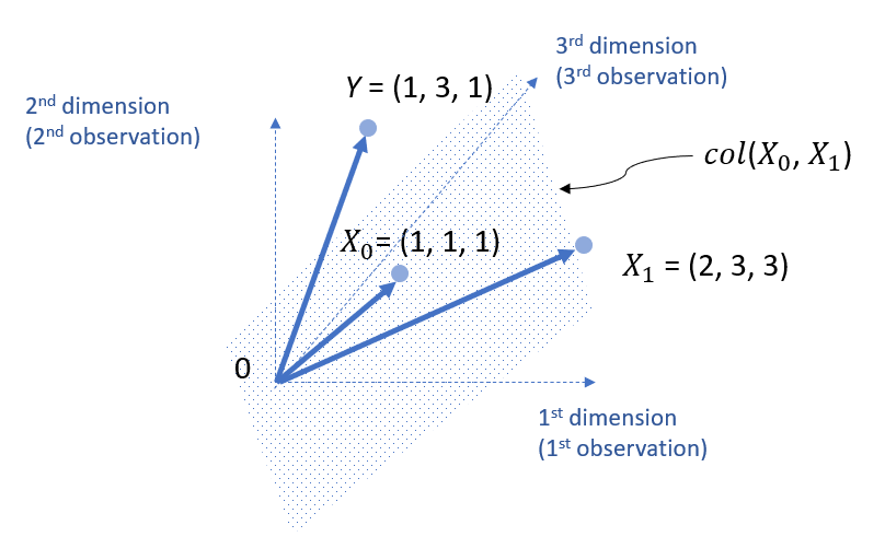
Note that, such a column space is not limited to two lines, but actually should be expanded beyond that. That is, the following is a more accurate visual representation.
Based on my tutorial on orthogonal projection, we know that that, to find a point on the column space is to find an orthogonal projected point. Mathematically, we can calculate it as follows.
\( b= (X^{T} \cdot X)^{-1} \cdot X^{T} \cdot Y \)
Thus,
\( b=\left[\begin{array}{ccc}
b_0 \\
b_1 \end{array}
\right] = (X^{T} \cdot X)^{-1} \cdot X^{T} \cdot Y =(\left[\begin{array}{ccc} 1 & 1 &1 \\ 2 & 3 & 3 \end{array}\right] \left[\begin{array}{ccc} 1 & 2\\ 1 & 3 \\ 1 & 3 \end{array}\right])^{-1} \left[\begin{array}{ccc} 1 & 1 &1 \\ 2 & 3 & 3 \end{array}\right] \left[\begin{array}{ccc} 1\\ 3 \\ 1 \end{array}
\right] =\left[\begin{array}{ccc}
-1 \\
1 \end{array}
\right] \)
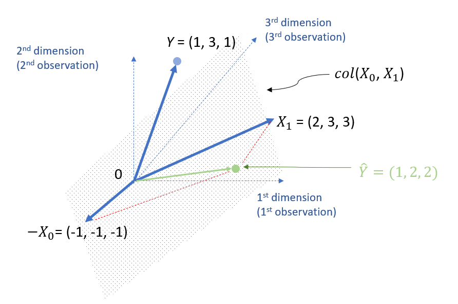
Thus, we can get \( \hat{Y} \) as follows.
\( \hat{Y}= -1*\left[\begin{array}{ccc} 1 \\ 1 \\ 1 \end{array} \right] +1* \left[\begin{array}{ccc} 2 \\ 3 \\ 3 \end{array} \right] = \left[\begin{array}{ccc} 1 \\ 2 \\ 2 \end{array} \right]\)
Thus, we can also plot it as follows.

You might wonder why the point of (1, 2, 2) is not between the arrow lines of X1 and X0. Actually, you can use the parallelogram law to draw the arrow lines for vectors. See below for the illustration.
I also used Andy Eggers’s R code to generate the following 3D visual representation. Unfortunately, I am not sure how to make it interactable on this website.
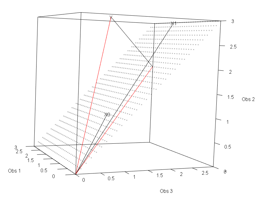
The following is the R code used to generate the figure above. The credit should go to Andy Eggers.
# R code to plot the projection for linear regression in 3D figure format

library(rgl)
constant <- c(1,1,1)
y <- c(1,3,1)
x <- c(2,3,3)
the_lm <- lm(y ~ x)

base_plot <- function(maxval = 3){
  plot3d(x = 0, y = 0, z = 0, type = "n",
         xlim = c(0,maxval),
         ylim = c(0,maxval),
         zlim = c(0,maxval),
         xlab = "Obs 1", ylab = "Obs 2", zlab = "Obs 3")
  text3d(x, texts = "X1")
  lines3d(x = rbind(c(0,0,0), x))
  text3d(constant, texts = "X0")
  lines3d(x = rbind(c(0,0,0), constant))
  text3d(y, texts = "Y")
  lines3d(x = rbind(c(0,0,0), y), col = "red")
}

base_plot()
df <- data.frame(rbind(x, constant, c(0,0,0)))
colnames(df) <- c("Obs 1", "Obs 2", "Obs 3")
plane_lm <- lm(`Obs 3` ~ `Obs 1` + `Obs 2`, data = rbind(df))
points_df <- expand.grid(x = seq(0, 3, .1), y = seq(0, 3, .1))
points_df$z <- coef(plane_lm)["`Obs 1`"]*points_df$x + coef(plane_lm)["`Obs 2`"]*points_df$y
points3d(points_df, alpha = .3)

points3d(points_df, alpha = .3)
the_pred <- predict(the_lm)
lines3d(rbind(c(0,0,0), the_pred), col = "red", lwd = .5)
lines3d(rbind(y, the_pred), col = "black", lwd = .5)
Reference
- You can refer to this online tutorial by Andy Eggers on the geometric interpretation of linear regression on the difference between rows and columns on dimensions.
- This tutorial is also inspired by Vladimir Mikulik‘s Why Linear Regression is a Projection (published on Medium), Thomas S. Robinson’s Chapter 3 Linear Projection, and Rafael Irizarry and Michael Love’s tutorial on projections.
Discussion