Conduct Paired Samples t-test in Excel
This tutorial shows detailed steps of how to do paired-sample t-test in Excel with a data example.
Data Example
The data table shown below has 3 columns, name, math, and English. We are going to compare if Math and English are significantly different.

Hypothesis
The followings are the null hypothesis and the alternative one for paired sample t-test.
- Null Hypothesis: Math and English scores do not differ from each other.
- Alternative Hypothesis: Math and English scores do differ from each other.
Step 1: Click “Data Analysis”
Next, click the “Data” menu and find the “Analysis” box. Then, click the “Data Analysis” module.
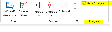
If you can not find the Data Analysis” module, please refer to another tutorial showing how to add “Data Analysis” to Excel.
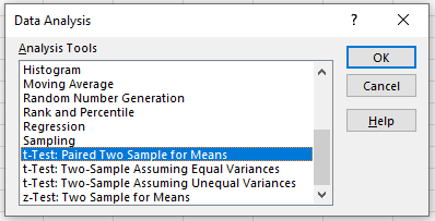
Step 2:
On the pop-up window, click the “t-Test: Paired Two Sample for Means” and then click “OK.”
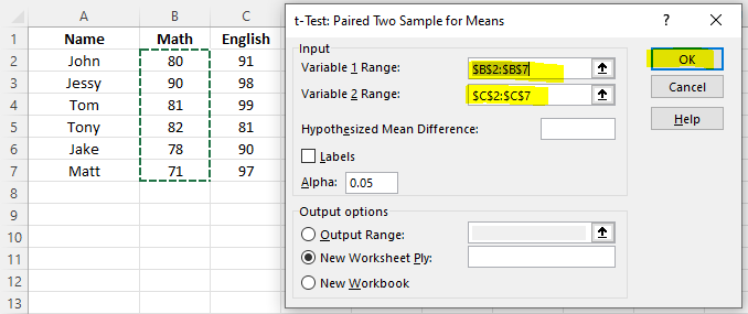
Step 3: Input Range
Select B2 to B7 to Variable 1 Range, and C2 to C7 to Variable 2 Range. Then, click “OK.”
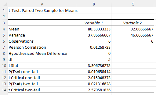
Step 4: Interpretation
The following is the output of Paired Samples t-test in Excel. We use the two-tail p-value, which is equal to 0.021, namely smaller than 0.05. Thus, we reject the null hypothesis and conclude that Math and English scores do differ from each other.
Discussion