Linear Mixed Models in SPSS

This tutorial includes the explanation of what a linear mixed model is, how to structure its statistical model, data example, as well as steps for linear mixed models in SPSS.

Definition of Linear Mixed Models

Linear mixed models (LMMs) are statistical models used to analyze data that have both fixed and random effects. They are an extension of linear regression models that incorporate random effects to account for correlation and variability within the data.

In a linear mixed model, the response variable is assumed to be influenced by both fixed effects and random effects. The fixed effects represent the average effect of the predictors on the response variable, while the random effects capture the individual variability or clustering within the data.

The fixed effects in a linear mixed model are similar to those in a standard linear regression model. They are typically represented by regression coefficients that estimate the average effect of the predictor variables on the response variable. These fixed effects are assumed to be constant across all individuals or groups in the data.

The random effects in a linear mixed model are used to account for the variability that is specific to different individuals or groups. These random effects are modeled as random variables with a specific distribution, such as a normal distribution. The random effects allow for the correlation within clusters or repeated measures within subjects.

To explain why we need linear mixed models, we can start with an example. For instance, to test how teaching methods (e.g., new vs. old) can impact scores, we can just do a simple t-test, ANOVA, or even simple linear regression. That is, typically, we do not consider the impact of students being from different schools (e.g., School A, School B, and School C, see below).

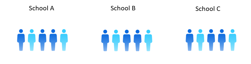
However, we can easily imagine that students from the same school would have similar scores. To address this, we can use mixed effects models, including fixed (teaching method) and random (schools) effects.

---

Statistical Model for Linear Mixed Models

The general form of a linear mixed effects model can be expressed as:

Y = Xβ + Zb + ε

where:

• Y is the response variable.
• X and Z are design matrices that represent the fixed effects and random effects, respectively.
• β represents the fixed effects coefficients.
• b represents the random effects coefficients.
• ε is the error term.

The fixed effects part of the model (Xβ) explains the relationships between the response variable and the fixed predictors, similar to a standard linear regression model. The random effects part (Zb) accounts for the variations between groups and incorporates the random predictors.

The random effects are assumed to follow a multivariate normal distribution with mean zero and a covariance matrix that reflects the structure of the data. The covariance structure allows for correlations between observations within the same group.

---

Data and Model

You can download the SPSS SAV file for linear mixed models here . (Note that, this is hypothetical data.)

In particular, suppose we are interested in examining the effect of a new teaching method on students’ test scores.

In this example, we want to assess the impact of the teaching method (fixed effect) while accounting for the variations between schools (random effect).

Student ID	School	Teaching Method	Test Score
1	A	Old	90
2	A	Old	90
3	A	New	100
4	B	Old	70
5	B	New	90
6	B	New	95
7	C	New	75
8	C	New	75
9	C	Old	60
10	D	Old	65
11	D	Old	65
12	D	New	70

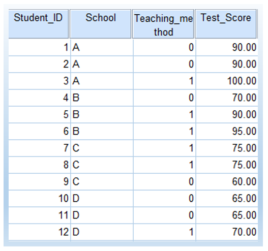
The following show how the data looks like in SPSS. 0 represents ‘old’ and 1 represents ‘new’ in Teaching_method.

The following is the model statement with both fixed effects and random effect.

Test Score = β₀ + β₁ * Teaching Method + b₀(School) + ε

where:

• β₀ and β₁ are the fixed effects coefficients representing the intercept and the effect of the teaching method, respectively.
• b₀(School) is the random effect for each school.
• ε is the error term.

---

Part 1: Fixed Effect Only

In this section, we are going to have a model with fixed effect only in SPSS.

Thus, basically it is a typical linear regression model without any random effects (see my other tutorials on simple linear regression and multiple linear regression).

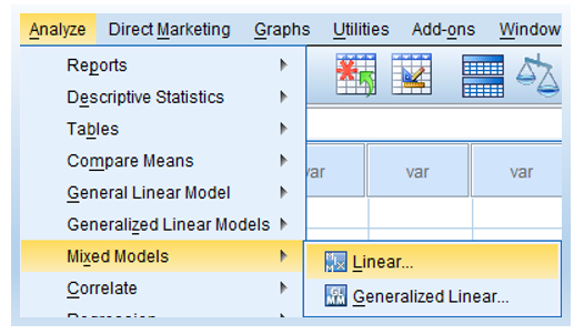
1. Click Analyze > Mixed Models > Linear, as shown below.
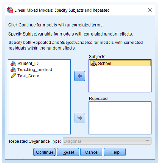
2. Not selecting any variables into subjects or repeated.
   
   We start with a fixed effect only model, which serves as a baseline model. Thus, we do NOT specify any random variable here. Just doing nothing with this window and click Continue.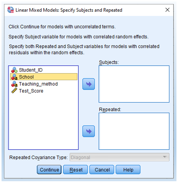
   
   
3. Move Test Score as Dependent Variable and Teaching method as Covariate(s).
   
   Note that, the estimates for slope and intercept would be inaccurate if Teaching method is put into the box of Factor(s). I am not sure why. Andy Field’s Discovering Statistics Using SPSS (E3 p. 744) footnote has a similar discussion.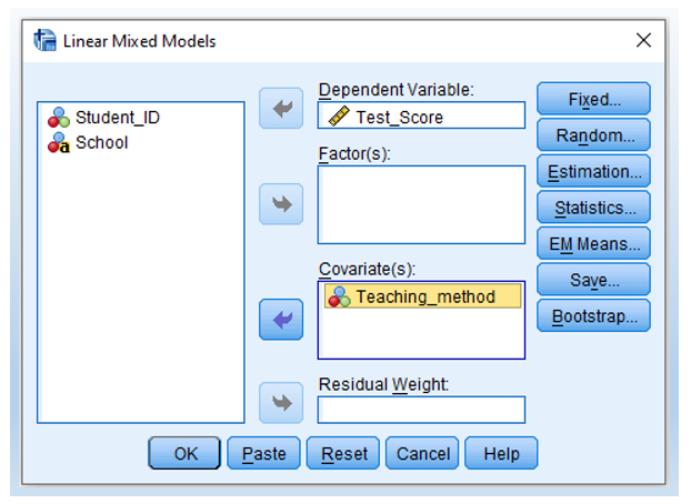
   
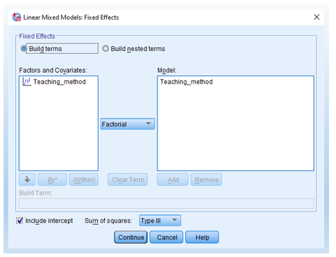
4. Then, click the Fixed button (shown above) and move Teaching method into the Model on the right-hand box (see below).
   
5. Click Estimation and then select Maximum Likelihood.
   
   According to Andy Field’s Discovering Statistics Using SPSS (E3 p. 746), if we want to do a model comparison, we need to select maximum likelihood (ML) rather than restricted maximum likelihood (REML).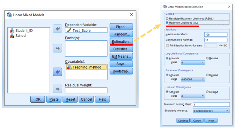
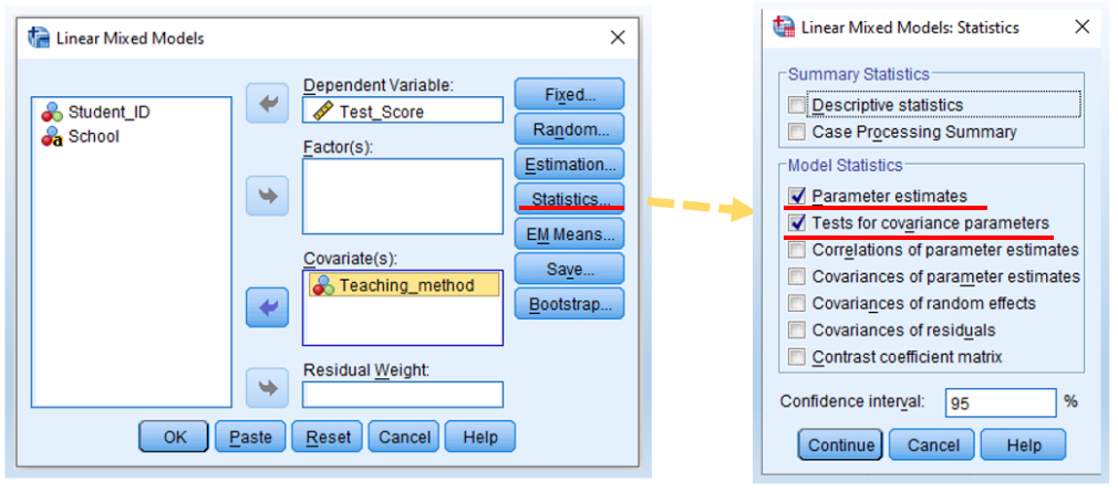
6. Click Statistics. Then, check Parameter estimates and Tests for covariance parameters. Then, click Continue and then OK.

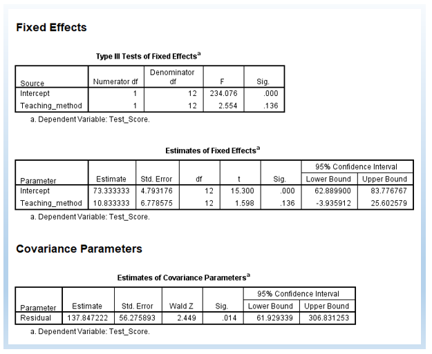
We can then see the following output. Note that the -2 Log Likelihood is 93.168. Note that, basically, we are doing a simple linear regression here, since we do not have any random effect.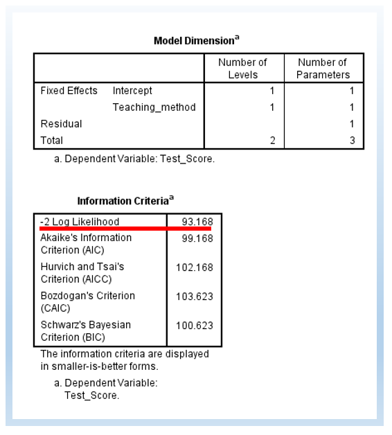

---

Part 2: Add Random Intercept

Extending the 5 steps shown above, we are going to add random intercept into the model. To do so, there are only 2 additional steps.

1. First, move School into Subjects. Thus, this is different from Step 2 shown earlier.
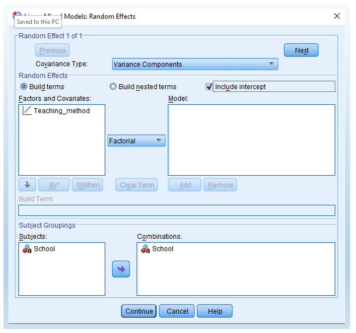
2. Second, click Include intercept in the Random Effects menu. Then, click OK and run it to see the results.

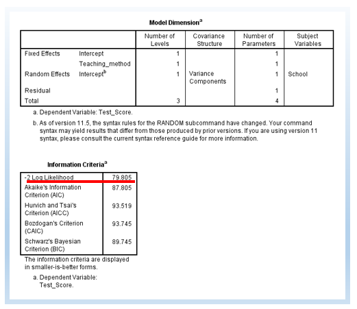
The following output is a model with a random intercept. First, there are 4 estimated parameters, rather than 3 Part 1. The -2 Log Likelihood is 79.805. The difference is 13.363. The change in degree of freedom (df) is 1.

χ² _change = 93.168-79.805=13.363
df _change = 4 – 3 = 1

13.362 is greater than 3.84 (p < .05), the critical value for chi-square distribution for the alpha level at .05 for the degree of freedom at 1. Thus, we can see that the random intercept model is significantly improving the model.

In the Information Criteria below, you can also see AIC, AICC, CAIC, and BIC. Typically, we use AIC and BIC to do model comparisons as well. The rule of thumb is that, smaller values mean better-fitting models. This is similar to -2 Log Likelihood such that a smaller value of -2 Log Likelihood means a better model.

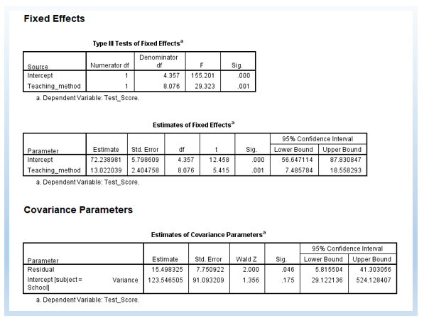
Further, we can see that the p-value for the slope became significant, p = .001. It was p = .136 in the fixed effect only model (i.e., in Part 1). Thus, we can see that, by adding the random intercept, we can get a different conclusion regarding the effectiveness of teaching methods on student score results.

You can also plot it in SPSS to plot it (see below). To keep this tutorial precise, I do not provide details regarding how to plot this figure. Regardless, the following is the plot, as we can see the slope is the same but the intercepts are different between schools.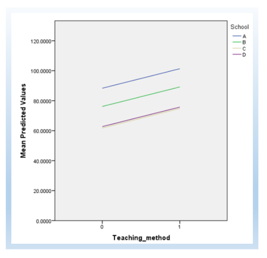

---

Part 3: Add Random Slope

Building on the top of the random intercept, we can also test the random slope. Thus, in Part 3, the model has both random intercepts and random slopes.

Basically, there are two additonal steps that you need to do.

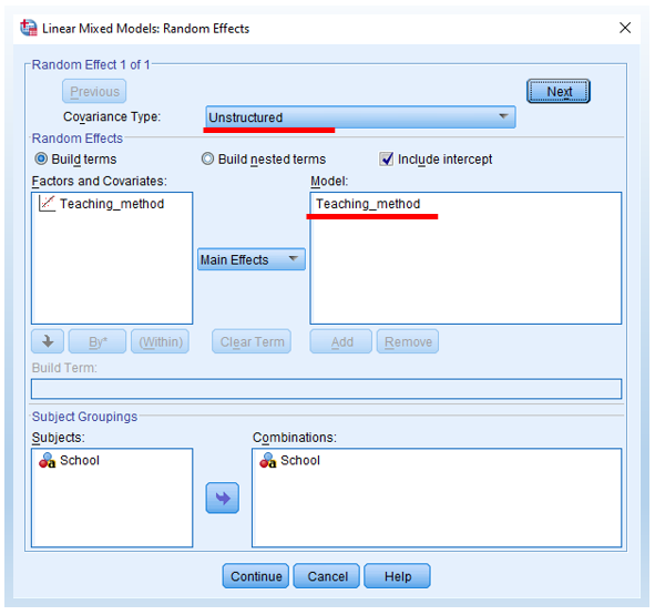
1. Add Teaching_method into the right-hand side Model box. It means that we add Teaching_method as the grouping variable for random slope (see below).
2. Change covariance type from Variance components to Unstructured (see below).

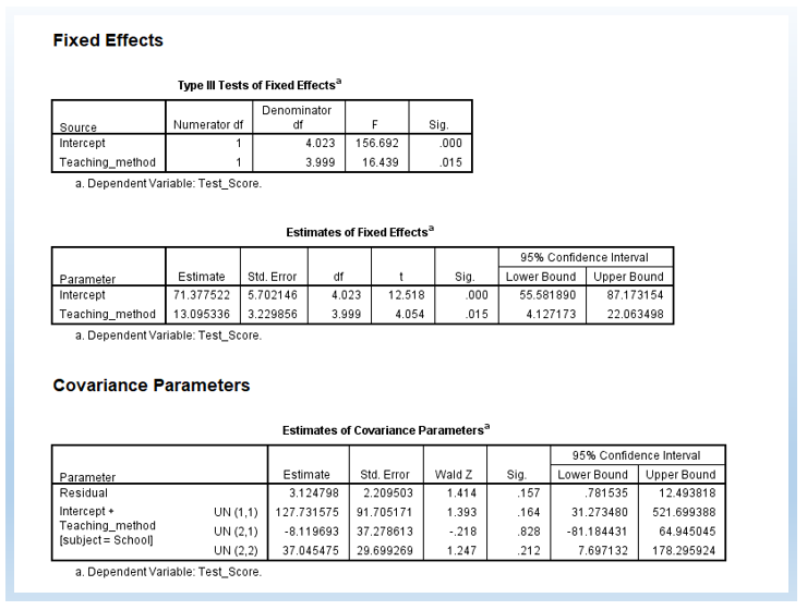
The following is the output with random slope and intercept. Now, we estimate 6 parameters. The difference in -2 Log Likelihood between random intercept only and random intercept + slope is 4.105. The difference in degree of freedom is 2.

χ² _change = 79.805 – 75.700 = 4.105
df _change = 6 – 4 = 2

4.105 is smaller than 5.991, the critical value for chi-square distribution for the alpha level at .05 for the degree of freedom at 2. Thus, statistically, we do not need to add the random slope into the model, and we could just just allow random intercept only in the model.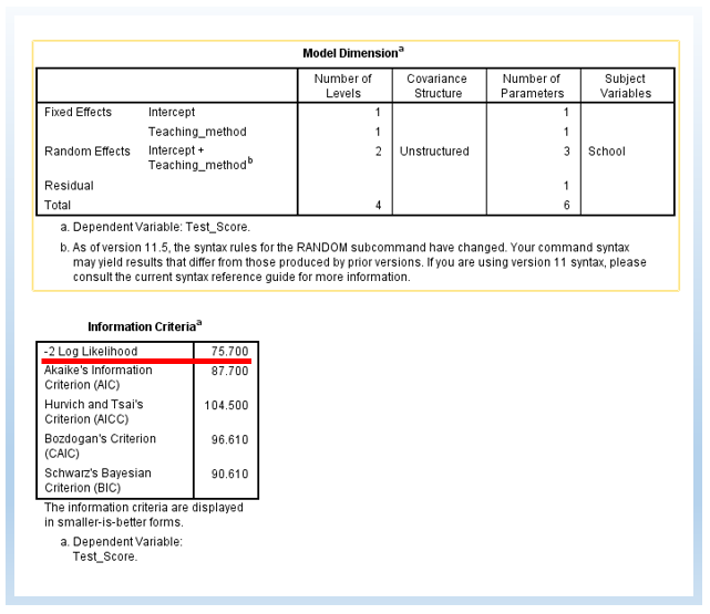


We can also plot the random intercept and slope as follows, to get a visual understanding. (The detailed steps of how to plot it are not provided in this tutorial.)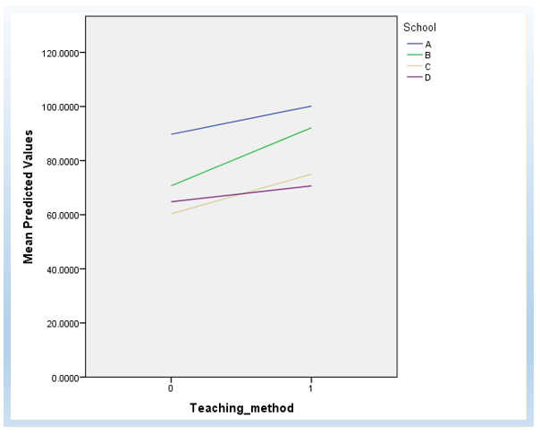

Of course, you can also test only random slopes without random intercepts. However, to control the length of this tutorial, I do not include that here.

---

Reference and Further Reading

The major reference I used in this tutorial was Andy Field’s Discovering Statistics Using SPSS (Chapter 19 Multilevel Linear Models E3). If you can not get Andy’s textbook, you can also refer to Matthew E. Clapham’s Linear mixed effects models on YouTube, which focuses on more the conceptual part. One point he mentions is important, if you only have 2 or 3 groups, you might not need to consider it as a grouping variable in linear mixed effect models, but rather you can just use it as a fixed effect (e.g., 2-way ANOVA).

Finally, you can also refer to Ayumi Shintani on Mixed Effect (Random Effect) in SPSS on YouTube, and she showed you how to step by step to conduct the analysis in SPSS. Just notice that her data has repeated measures, and in contrast, the data in my tutorial does not have repeated measures.

I also have another tutorial on maximum likelihood estimation (MLE) for linear regression.